
Lab B: Graphical model stability and variable selection procedures with mplot
Samuel Müller and Garth Tarr
Learning outcomes
- Cross validation with the
caretpackage - The
mplotpackage - Variable inclusion plots
- Model stability plots
- Bootstraping the lasso
Required R packages:
install.packages(c("mplot", "pairsD3", "Hmisc", "caret"))Body fat data
In lab A we found that both forward and backward stepwise methods selected the same model Fore, Neck, Weight and Abdo. An F test “confirmed” that this was better than a simple linear regression of Bodyfat on Abdo, however this was all done “in-sample”. It may be of interest to compare these two models on their out-of-sample predictive ability using cross validation with the caret package.
library(caret)
data("bodyfat", package = "mplot")
# help('bodyfat', package = 'mplot')
names(bodyfat)
## [1] "Id" "Bodyfat" "Age" "Weight" "Height" "Neck" "Chest"
## [8] "Abdo" "Hip" "Thigh" "Knee" "Ankle" "Bic" "Fore"
## [15] "Wrist"bfat = bodyfat[, -1] # remove the ID column
# specify how we want the cross validation to run
set.seed(2)
control = trainControl(method = "cv", number = 10)
lm4_cv = train(Bodyfat ~ Fore + Neck + Weight + Abdo, method = "lm", data = bfat,
trControl = control)
lm4_cv## Linear Regression
##
## 128 samples
## 4 predictor
##
## No pre-processing
## Resampling: Cross-Validated (10 fold)
## Summary of sample sizes: 116, 116, 115, 115, 114, 115, ...
## Resampling results:
##
## RMSE Rsquared MAE
## 4.009105 0.7698252 3.231992
##
## Tuning parameter 'intercept' was held constant at a value of TRUElm1_cv = train(Bodyfat ~ Abdo, method = "lm", data = bfat, trControl = control)
lm1_cv## Linear Regression
##
## 128 samples
## 1 predictor
##
## No pre-processing
## Resampling: Cross-Validated (10 fold)
## Summary of sample sizes: 116, 114, 114, 115, 115, 116, ...
## Resampling results:
##
## RMSE Rsquared MAE
## 4.200029 0.734844 3.384656
##
## Tuning parameter 'intercept' was held constant at a value of TRUEresults <- resamples(list(lm4 = lm4_cv, lm1 = lm1_cv))
summary(results)##
## Call:
## summary.resamples(object = results)
##
## Models: lm4, lm1
## Number of resamples: 10
##
## MAE
## Min. 1st Qu. Median Mean 3rd Qu. Max. NA's
## lm4 2.139669 2.571588 3.311596 3.231992 3.597563 4.461380 0
## lm1 2.603673 2.804505 3.326438 3.384656 3.795808 4.877285 0
##
## RMSE
## Min. 1st Qu. Median Mean 3rd Qu. Max. NA's
## lm4 3.040804 3.294321 3.955285 4.009105 4.462737 5.405007 0
## lm1 3.081008 3.842363 4.075765 4.200029 4.624086 5.941870 0
##
## Rsquared
## Min. 1st Qu. Median Mean 3rd Qu. Max. NA's
## lm4 0.6148935 0.7613316 0.7848377 0.7698252 0.8046156 0.8876280 0
## lm1 0.5968823 0.7053104 0.7555442 0.7348440 0.7710089 0.8227845 0library(ggplot2)
ggplot(results) + theme_classic() + labs(y = "MAE")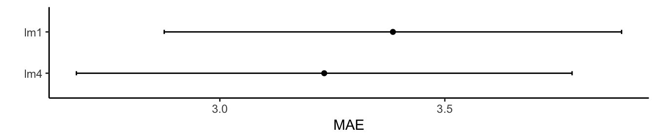
ggplot(results, metric = "RMSE") + theme_classic() + labs(y = "RMSE")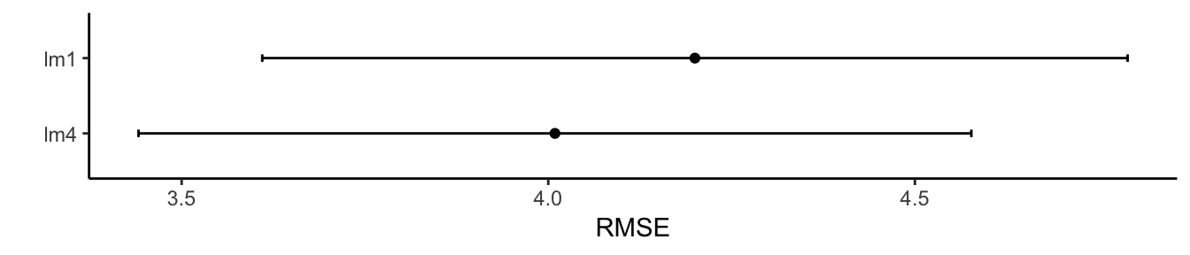
ggplot(results, metric = "Rsquared") + theme_classic() + labs(y = "R-squared")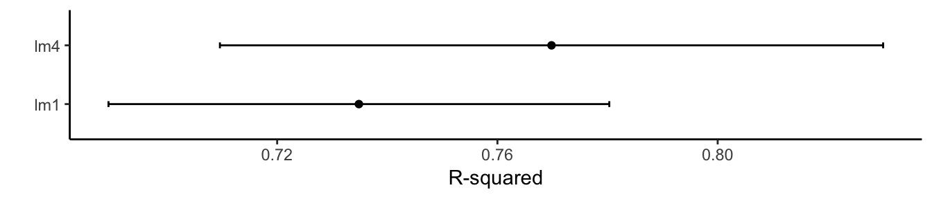
Your turn: Repeat the above, but perform repeated 5-fold cross validation with 10 repeats. Hint: in the trainControl() function use the repeats argument.
control = trainControl(method = "repeatedcv", number = 5, repeats = 10)
lm4_cv = train(Bodyfat ~ Fore + Neck + Weight + Abdo, method = "lm", data = bfat,
    trControl = control)
lm1_cv = train(Bodyfat ~ Abdo, method = "lm", data = bfat, trControl = control)
results <- resamples(list(lm4 = lm4_cv, lm1 = lm1_cv))
ggplot(results) + theme_classic() + labs(y = "MAE")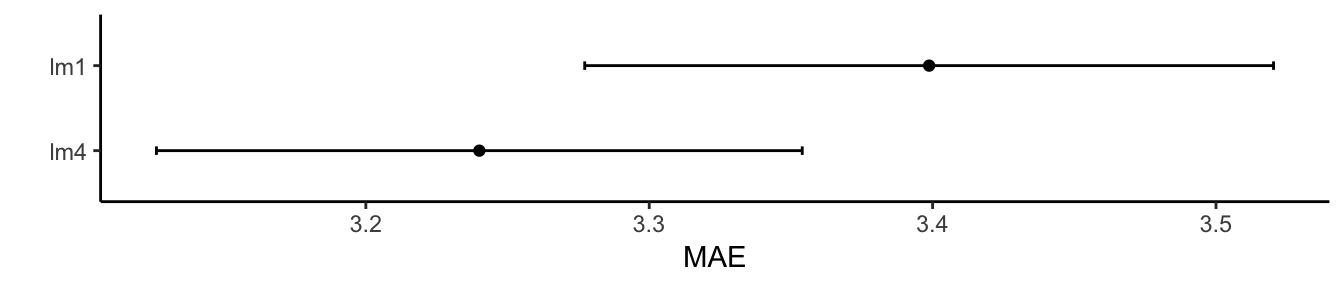
ggplot(results, metric = "RMSE") + theme_classic() + labs(y = "RMSE")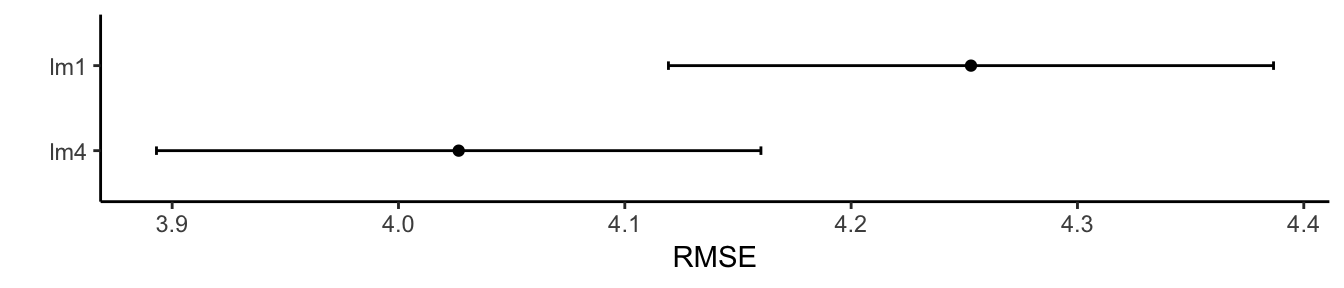
ggplot(results, metric = "Rsquared") + theme_classic() + labs(y = "R-squared")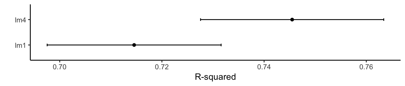
For further information about the caret package see here.
Diabetes data
Start exploring the diabetes example through the demonstrator version of the shiny interface that can be obtained through mplot() either by loading http://garthtarr.com/apps/mplot/ or by using the code below.
library(mplot)
load(url("http://garthtarr.com/dbeg2019.RData"))
# makes available objects full.mod, af1,v1 and bgn1
mplot(full.mod, af1, v1, bgn1)
# mplot takes as an input a full model in its first slot and then one or more
# objects of type vis, af or bglmnet
# this code was used to create the dbeg2019.RData object DON'T run it on your
# laptop, as it may take some time to complete library(mplot) data(diabetes)
# full.mod = lm(y ~ ., data = diabetes) af1 = af(full.mod, B = 200, n.c = 150,
# c.max = 100) v1 = vis(full.mod, B = 200, nbest = 'all') bgn1 =
# bglmnet(full.mod, B = 200) save(file = 'dbeg2019.RData', full.mod, af1, v1,
# bgn1)If there is no left black sidebar, click in the blue heading on the menu/sidebar icon.
1. Explore visually the ‘Variable inclusion’ plot and do the following:
- Hover over the green colored hdl curve in the right ‘label panel’: the entire curve is rendered in bold.
- Why does this hdl curve have a different behaviour (non-monotone decreasing) to the other curves (who are monotone decreasing)?
- Hover over the purple colored RV curve in the right panel: This curve shows an example-curve for a variable that is known to be redundant (alternative expressions are not-important or not-predictive).
- What do you conclude for curves (variables) that are close to this mint colored RV curve?
- Confirm that the bootstrapped/empirical probability of selecting tc is 0.87 (2dp) when a AIC penalty of \(\lambda=2\) is selected and that the bootstrapped probability of selection decreases to 0.59 (2dp) if a BIC penalty, ie \(\lambda=\log(n)\), is selected instead.
- Render a non-interactive version of the variable inclusion plot by clicking ‘No’ under the ‘Interactive plots’ heading in the left sidebar.
2. Explore the ‘Bootstrap glmnet’ tab next (for the diabetes example, we can easily do an exhaustive variable inclusion plot as seen above; however, in general, this may not be feasible, so bootstrapping glmnet will be more feasible):
- Confirm that hdl has again a different behaviour (as seen above) to the other curves (although ldl is also somewhat different: both hdl and ldl are cholesterol measurements https://en.wikipedia.org/wiki/Cholesterol) .
- Confirm that the ordering of the variables according to their ‘importance’, estimated through the bootstrapped probability, is very similar for this plot as for the variable inclusion plot before.
- Confirm that four variables have a bootstrapped probability that is larger than 50% when the penalty parameter is 10. Confirm that this is the same number of variables in the variable inclusion plot that have a bootstrapped probability exceeding 50% when \(\lambda=10\).
Revisit Crime data from Lab A: explore subtractive measures
Read in the dataset UScrime from the MASS package and fit a full model (called M1). Note that you can access the t-statistic values by returning the third column from M1.sum$coefficients where M1.sum = summary(M1)
data("UScrime", package = "MASS")
M1 = lm(y ~ ., data = UScrime)  # Full model
M1.sum = summary(M1)
M1.sum$coefficients
## Estimate Std. Error t value Pr(>|t|)
## (Intercept) -5984.2876045 1628.3183733 -3.67513362 0.0008929887
## M 8.7830173 4.1713866 2.10553902 0.0434433942
## So -3.8034503 148.7551399 -0.02556853 0.9797653725
## Ed 18.8324315 6.2088376 3.03316541 0.0048614327
## Po1 19.2804338 10.6109676 1.81702882 0.0788919769
## Po2 -10.9421925 11.7477536 -0.93142851 0.3588295738
## LF -0.6638261 1.4697288 -0.45166573 0.6546540941
## M.F 1.7406856 2.0353843 0.85521225 0.3989953316
## Pop -0.7330081 1.2895554 -0.56841928 0.5738452309
## NW 0.4204461 0.6480892 0.64874725 0.5212791189
## U1 -5.8271027 4.2102890 -1.38401489 0.1762380311
## U2 16.7799672 8.2335955 2.03798780 0.0501612829
## GDP 0.9616624 1.0366605 0.92765416 0.3607537824
## Ineq 7.0672099 2.2716521 3.11104410 0.0039831365
## Prob -4855.2658155 2272.3746212 -2.13664850 0.0406269260
## Time -3.4790178 7.1652752 -0.48553862 0.6307084351M1.sum$coefficients[, 3]## (Intercept) M So Ed Po1 Po2
## -3.67513362 2.10553902 -0.02556853 3.03316541 1.81702882 -0.93142851
## LF M.F Pop NW U1 U2
## -0.45166573 0.85521225 -0.56841928 0.64874725 -1.38401489 2.03798780
## GDP Ineq Prob Time
## 0.92765416 3.11104410 -2.13664850 -0.48553862Note that the regression coefficient for Prob is very large but also its corresponding standard error is very large; additionally, the standard errors vary considerably from variable to variable.
Copy and paste the sstab function from Lecture B, then modify it to generate \(B=200\) weighted bootstrap t statistics, that is standardizing estimated regression coefficients by dividing this with their standard error, store this matrix in an object called sstab.out.
sstab = function(mf, B = 100) {
    full_coeff = coefficients(mf)
    kf = length(full_coeff)
    coef.res = matrix(ncol = kf, nrow = B)
    colnames(coef.res) = names(full_coeff)
    formula = stats::formula(mf)
    data = model.frame(mf)
    for (i in 1:B) {
        wts = stats::rexp(n = length(resid(mf)), rate = 1)
        data$wts = wts
        mod = stats::lm(formula = formula, data = data, weights = wts)
        coef.res[i, ] = summary(mod)$coefficients[, 3]  # only change is here
    }
    return(coef.res)
}

sstab.out = sstab(M1, B = 200)
head(sstab.out)
## (Intercept) M So Ed Po1 Po2
## [1,] -2.894650 1.745907 1.0096499 3.4817995 1.42330930 -0.20789800
## [2,] -5.210971 2.329495 0.7729234 3.6595162 2.61512960 -1.87667149
## [3,] -3.954544 1.356865 -0.3684651 0.8016911 0.03890622 0.44090500
## [4,] -2.886448 2.237135 0.8571393 2.5738202 0.17367777 0.61791387
## [5,] -4.735308 1.766034 1.6000960 2.7481889 0.88763461 -0.02890344
## [6,] -4.355798 2.765337 -0.9204242 3.0211384 0.01932286 0.47730378
## LF M.F Pop NW U1 U2
## [1,] -0.75556797 0.6118904 0.18205055 -0.4851379 -1.6317948 1.626705
## [2,] -0.91189296 1.2626159 0.50276929 0.7763823 -0.6266095 1.540590
## [3,] 0.06392066 1.5519286 -0.04019839 1.0740166 -1.3236990 1.536783
## [4,] 1.15518094 -0.2114486 -0.66686094 0.1600191 -1.1127974 2.322563
## [5,] 0.65122118 2.1177486 -1.20018342 0.6170354 -1.3600375 2.681239
## [6,] -0.66230677 0.3891202 -0.56008895 -0.4176735 -2.1765896 3.078368
## GDP Ineq Prob Time
## [1,] 0.4664786 3.604550 -2.566126 -0.46414032
## [2,] 2.0301164 4.291281 -2.371420 -0.99428972
## [3,] 1.7830890 2.447188 -1.603865 -0.05799234
## [4,] 0.3231917 2.504817 -1.987240 -0.55929460
## [5,] -0.9819544 1.477717 -1.377223 1.56420094
## [6,] 2.0984415 5.917044 -1.715784 0.49831627Calculate the absolute values of the bootstrapped t-statistics, delete the first column (the values for the intercept) and store it in an object called sj.
sj = abs(sstab.out[, -1])
head(sj)
## M So Ed Po1 Po2 LF M.F
## [1,] 1.745907 1.0096499 3.4817995 1.42330930 0.20789800 0.75556797 0.6118904
## [2,] 2.329495 0.7729234 3.6595162 2.61512960 1.87667149 0.91189296 1.2626159
## [3,] 1.356865 0.3684651 0.8016911 0.03890622 0.44090500 0.06392066 1.5519286
## [4,] 2.237135 0.8571393 2.5738202 0.17367777 0.61791387 1.15518094 0.2114486
## [5,] 1.766034 1.6000960 2.7481889 0.88763461 0.02890344 0.65122118 2.1177486
## [6,] 2.765337 0.9204242 3.0211384 0.01932286 0.47730378 0.66230677 0.3891202
## Pop NW U1 U2 GDP Ineq Prob
## [1,] 0.18205055 0.4851379 1.6317948 1.626705 0.4664786 3.604550 2.566126
## [2,] 0.50276929 0.7763823 0.6266095 1.540590 2.0301164 4.291281 2.371420
## [3,] 0.04019839 1.0740166 1.3236990 1.536783 1.7830890 2.447188 1.603865
## [4,] 0.66686094 0.1600191 1.1127974 2.322563 0.3231917 2.504817 1.987240
## [5,] 1.20018342 0.6170354 1.3600375 2.681239 0.9819544 1.477717 1.377223
## [6,] 0.56008895 0.4176735 2.1765896 3.078368 2.0984415 5.917044 1.715784
## Time
## [1,] 0.46414032
## [2,] 0.99428972
## [3,] 0.05799234
## [4,] 0.55929460
## [5,] 1.56420094
## [6,] 0.49831627Calculate the mean rank of the absolute t-values (copy and paste from the lecture) and note that Ineq and Ed have highest rank.
sj_ranks = apply(sj, 1, rank)
sj_rank_mean = sort(apply(sj_ranks, 1, mean), decreasing = TRUE)
sj_rank_mean
## Ineq Ed U2 Prob M Po1 U1 M.F GDP Po2 Time
## 13.785 13.290 10.715 10.705 10.665 9.480 8.325 6.750 6.365 5.710 5.285
## NW Pop LF So
## 5.110 4.770 4.760 4.285Produce a variable inclusion plot and a bootstrapped loss versus dimension plot, can you confirm the above observation?
library(mplot)
vis.out = vis(M1)
##
## Using nbest = "all" is not currently allowed when the full
## model has more than 15 variables. Defaulting to nbest = 1
## plot(vis.out, which = "vip", interactive = TRUE)## Creating a generic function for 'toJSON' from package 'jsonlite' in package 'googleVis'plot(vis.out, which = "boot", interactive = TRUE)Solid waste data of Gunst and Mason (1980)
This is a famous design matrix, often used to test variable selection methods. Here \(n=40\) and the number of slopes (explanatory variables) is \(k=4\), the total number of regression parameters is therefore \(p=5\). The design matrix is available in the bestglm package.
data("Shao", package = "bestglm")
X = as.matrix.data.frame(Shao)
Confirm that the number of rows and columns are 40 and 4, respectively using the function dim (alternatively you could use the functions ncol or nrow).
dim(X)## [1] 40 4ncol(X)## [1] 4nrow(X)## [1] 40Return the first few rows of the design matrix \(X\) using the command head and note that it has not yet a column of ones representing the intercept.
head(X)## x2 x3 x4 x5
## [1,] 0.36 0.53 1.06 0.5326
## [2,] 1.32 2.52 5.74 3.6183
## [3,] 0.06 0.09 0.27 0.2594
## [4,] 0.16 0.41 0.83 1.0346
## [5,] 0.01 0.02 0.07 0.0381
## [6,] 0.02 0.07 0.07 0.3440In the literature, the intercept is often chosen to be \(\beta_0 = 2\) and four data generating slope vectors are frequently used for this data: \(\boldsymbol{\beta}_{\text{slopes}}^T = (0,0,4,0)\), \((0,0,4,8)\), \((9,0,4,8)\) or \((9,6,4,8)\).
We continue with looking at the smaller of the two intermediate cases, choosing \[\boldsymbol{\beta}^T=(2,0,0,4,8).\] The other three choices as well as variations thereof can be done later in the lab.
The data generating model is \[\pmb{y} = \pmb{X}\pmb{\beta} + \pmb{\epsilon},\] with \(\pmb{\epsilon} \sim N(\pmb{0},\pmb{I})\).
To have reproducable results, set the random seed to 2 (it’s the second tutorial), generate the response vector \(\pmb{y}\), by y = 2 + X %*% c(0,0,4,8) + rnorm(n), note that %*% multiplies the matrix \(\pmb{X}\) with the (column) vector \(\pmb{\beta}\) and rnorm(n) generates \(n\) standard normal distributed pseudo-random numbers.
set.seed(2)
n = 40
y = 2 + X %*% c(0, 0, 4, 8) + rnorm(n)
Next, fit the full model using lm. Store the full model in an R object called lm.full and then produce its summary output.
lm.full = lm(y ~ X)
summary(lm.full)
##
## Call:
## lm(formula = y ~ X)
##
## Residuals:
## Min 1Q Median 3Q Max
## -2.51914 -0.46378 0.08213 0.57235 2.05907
##
## Coefficients:
## Estimate Std. Error t value Pr(>|t|)
## (Intercept) 2.0783 0.2272 9.148 8.27e-11 ***
## Xx2 2.8418 1.9707 1.442 0.158
## Xx3 -1.0662 1.0690 -0.997 0.325
## Xx4 4.4082 0.6157 7.160 2.38e-08 ***
## Xx5 7.1284 0.4887 14.586 < 2e-16 ***
## ---
## Signif. codes: 0 '***' 0.001 '**' 0.01 '*' 0.05 '.' 0.1 ' ' 1
##
## Residual standard error: 1.115 on 35 degrees of freedom
## Multiple R-squared: 0.9917, Adjusted R-squared: 0.9908
## F-statistic: 1047 on 4 and 35 DF, p-value: < 2.2e-16Confirm that there are three highly significant variables, ‘unsurprisingly’ the (Intercept), Xx4 and Xx5.
Weighted bootstrap
Many fitting functions have a weights option, which can be used to implement the weighted bootstrap. A simple way to achieve this is by drawing repeatedly exponential bootstrap weights through w = rexp(n).
As an aside, the vector w has length n, with non-negative elements (the weights) that approximately sum to a number close to n.
First, observe what happens for a single run of the weighted boostrap, by reweighing observations with w and storing the output of lm(y~X, weights=w) in the R object lm.full.b.
w = rexp(n)
length(w)  # is of course n=40
## [1] 40sum(w) # is approximately 40## [1] 42.2636lm.full.b = lm(y ~ X, weights = w)
summary(lm.full.b)##
## Call:
## lm(formula = y ~ X, weights = w)
##
## Weighted Residuals:
## Min 1Q Median 3Q Max
## -4.3058 -0.4663 0.0280 0.5404 2.9579
##
## Coefficients:
## Estimate Std. Error t value Pr(>|t|)
## (Intercept) 2.1403 0.2226 9.617 2.33e-11 ***
## Xx2 1.1906 2.7656 0.430 0.669
## Xx3 -1.1849 1.0214 -1.160 0.254
## Xx4 4.7641 0.7991 5.962 8.66e-07 ***
## Xx5 7.2679 0.5683 12.788 9.46e-15 ***
## ---
## Signif. codes: 0 '***' 0.001 '**' 0.01 '*' 0.05 '.' 0.1 ' ' 1
##
## Residual standard error: 1.122 on 35 degrees of freedom
## Multiple R-squared: 0.9874, Adjusted R-squared: 0.986
## F-statistic: 687.2 on 4 and 35 DF, p-value: < 2.2e-16Explore the weighted bootstrap next.
Observe how the coefficient values change for the full model above over initially \(B=10\) bootstrap samples (consider \(B=100\) and \(B=1000\) later, to see what changes and what more can be learned as \(B\) grows).
To achieve this, we repeat the above \(B\) times by writing a for loop and storing the coefficient vectors in the rows of a \(B\times p\) coefficient matrix C. (If you are a loop-novice and want to know more, you could work through https://www.datacamp.com/community/tutorials/tutorial-on-loops-in-r)
Store these coefficient values in a \(B\times p\) matrix C and return C by typing the following code:
B = 10
C = matrix(nrow = B, ncol = 5)
for (b in 1:B) {
    w = rexp(n)  # is inside the loop, otherwise weights don't change
    lm.full.b = lm(y ~ X, weights = w)
    C[b, ] = round(coef(lm.full.b), 2)
}
colnames(C) = c("Intcpt", "Slope_1", "Slope_2", "Slope_3", "Slope_4")
C
## Intcpt Slope_1 Slope_2 Slope_3 Slope_4
## [1,] 2.17 2.09 -0.90 4.29 7.32
## [2,] 1.97 2.37 -1.45 4.42 7.50
## [3,] 1.94 0.53 -0.61 4.27 7.82
## [4,] 2.04 4.79 -2.31 4.63 6.94
## [5,] 1.99 0.97 0.29 3.95 7.65
## [6,] 1.77 -0.41 1.00 4.17 7.40
## [7,] 1.79 2.92 -0.43 4.53 6.82
## [8,] 2.04 3.30 -1.37 4.23 7.29
## [9,] 2.00 3.81 -1.68 4.59 6.95
## [10,] 2.16 1.29 -0.95 4.37 7.62Next, calculate for each column (showing the bootstrapped regression coefficients) their standard deviation (using sd) and draw a boxplot of the coefficient estimates.
To apply a function to every column of a matrix C, use the apply function. (If you are a apply-novice and want to know more, you could work through https://www.datacamp.com/community/tutorials/r-tutorial-apply-family)
apply(C, 2, sd)## Intcpt Slope_1 Slope_2 Slope_3 Slope_4
## 0.1323338 1.5986119 0.9671660 0.2082333 0.3364339boxplot(C, horizontal = TRUE)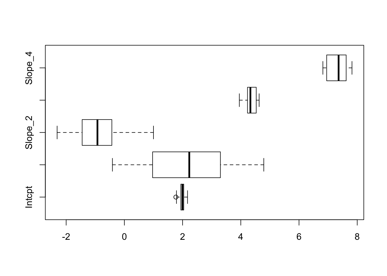
We observe that the first slope in particular varies a lot over the bootstrap sample, partly explained by the correlation structure in the data. Check the scatterplot (e.g. with pairs) and correlation matrix (e.g. with cor) to confirm: as an input to these two functions use the data frame dat = data.frame(y,X).
dat = data.frame(y, X)
pairs(dat)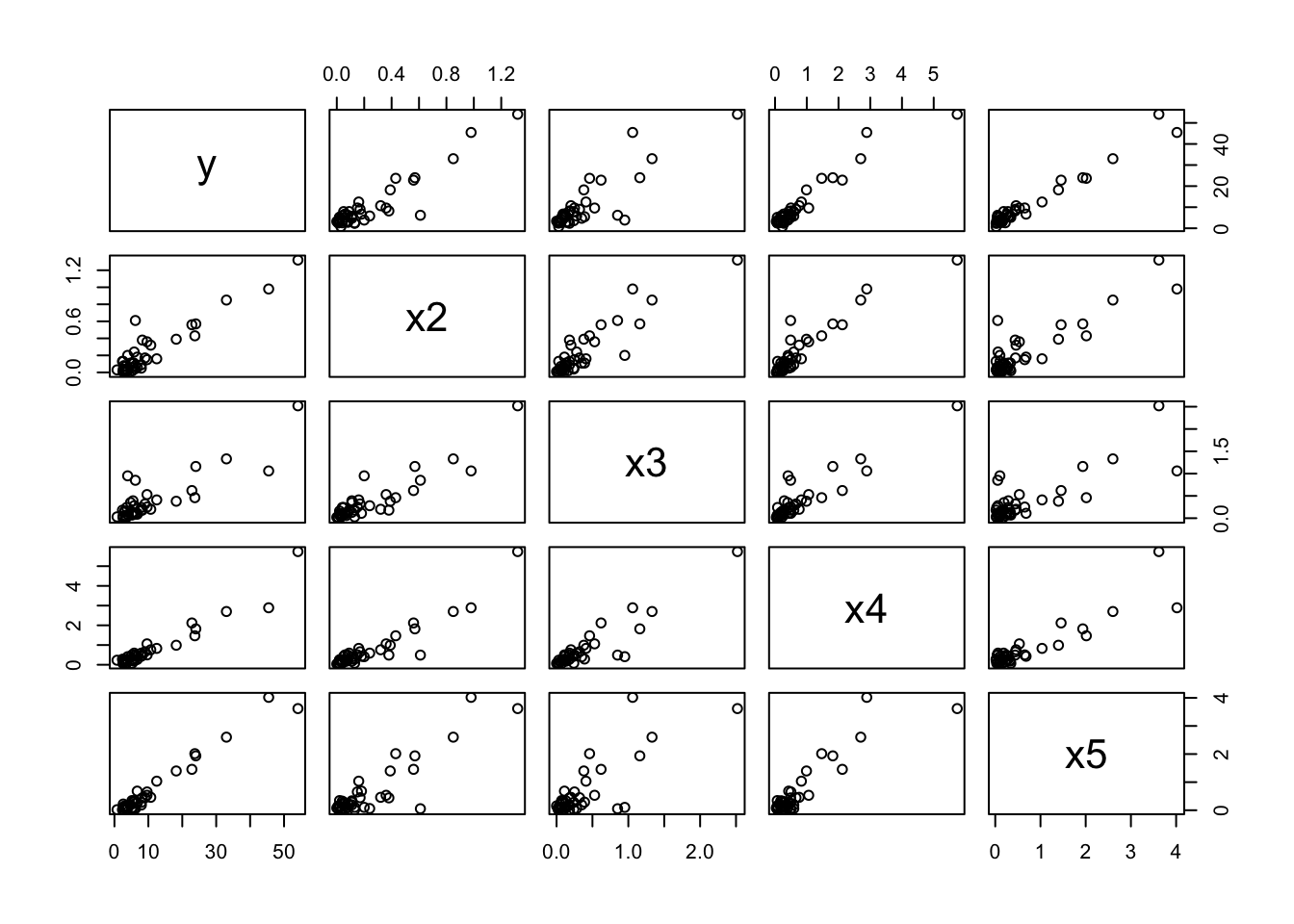
cor(dat)## y x2 x3 x4 x5
## y 1.0000000 0.9280339 0.8553656 0.9595148 0.9801890
## x2 0.9280339 1.0000000 0.9076253 0.9286497 0.8881846
## x3 0.8553656 0.9076253 1.0000000 0.9154477 0.7918901
## x4 0.9595148 0.9286497 0.9154477 1.0000000 0.9021348
## x5 0.9801890 0.8881846 0.7918901 0.9021348 1.0000000Calculate the bootstrap means of the coefficiencts (columns of C) and compare these values to the estimated coefficients for the full model above and the true parameter vector. Note that the bootstrapped values are approximately unbiased for the estimated coefficients but not for the true coefficient values.
C2 = cbind(c(2, 0, 0, 4, 8), round(coef(lm.full), 2), apply(C, 2, mean))
colnames(C2) = c("True", "Estimated", "Bootstraped")
C2
## True Estimated Bootstraped
## (Intercept) 2 2.08 1.987
## Xx2 0 2.84 2.166
## Xx3 0 -1.07 -0.841
## Xx4 4 4.41 4.345
## Xx5 8 7.13 7.331Repeat the above but change the number of bootstrap replications to \(B=100\) and then to \(B=1000\).
Further reading: The R packages boot and bootstrap both have functions to implement different versions of the regression bootstrap.
Three types of plots with vis()
Produce the three types of plots with the default values of the vis() function in the R package mplot. Store the output of vis in vis.out.
Check help(plot.vis) and note that the types of plots are which = c("vip", "lvk", "boot").
By default, the vis() function adds a sixth additional redundant variable. Reproduce the plots, setting redundant = FALSE.
Note: if you’re using markdown and you want the mplot plots to appear, you need to specify results='asis' in the chunck options and add tag="chart" to the parameters of the plot() call.
library(mplot)
vis.out = vis(lm.full)
plot(vis.out, which = "vip", interactive = TRUE)plot(vis.out, which = "lvk", interactive = TRUE)plot(vis.out, which = "boot", interactive = TRUE)Without the redundant variable.
vis.out2 = vis(lm.full, redundant = FALSE)plot(vis.out2, which = "vip", interactive = TRUE)plot(vis.out2, which = "lvk", interactive = TRUE)plot(vis.out2, which = "boot", interactive = TRUE)Different data generating models
Explore what changes when the size of the data generating model changes, that is choosing \(\boldsymbol{\beta}_{\text{slopes}}^T = (0,0,4,0)\), \((9,0,4,8)\) or \((9,6,4,8)\)
Clearly, the coefficients are all fairly large compared to the error standard deviation, which is \(\sigma=1\). Explore what happens above when choosing rescaled slopes, in particular for \(\boldsymbol{\beta}_{\text{slopes}}^T/2\) and \(\boldsymbol{\beta}_{\text{slopes}}^T/4\).
Bootstrapping the lasso
Even though for this small data set exhaustive searches are the natural way to do model selection, we explore the bglmnet() function. Among others, we can get the variable inclusion plot from learning only from the models on the bootstraped lasso paths.
To begin with, use the first simulaion setting with \(\pmb{\beta}^T = (2,0,0,4,8)\).
bglmnet.out = bglmnet(lm.full)plot(bglmnet.out, which = "vip", interactive = TRUE)