
Lab A: Introduction to model selection
Samuel Müller and Garth Tarr
Learning outcomes
- Stepwise methods
- Exhaustive searches
- Regularisation procedures
- Marginality
Required R packages
install.packages(c("mplot", "lmSubsets", "bestglm", "car", "ISLR", "glmnet", "MASS", "readr", "dplyr", "Hmisc","skimr", "mfp"))Stepwise methods
Diabetes
Efron et al. (2004) introduced the diabetes data set with 442 observations and 11 variables. It is often used as an examplar data set to illustrate new model selection techniques. The following commands will help you get a feel for the data.
data("diabetes", package="mplot")
# help("diabetes", package="mplot")
str(diabetes) # structure of the diabetes
## 'data.frame': 442 obs. of 11 variables:
## $ age: int 59 48 72 24 50 23 36 66 60 29 ...
## $ sex: int 2 1 2 1 1 1 2 2 2 1 ...
## $ bmi: num 32.1 21.6 30.5 25.3 23 22.6 22 26.2 32.1 30 ...
## $ map: num 101 87 93 84 101 89 90 114 83 85 ...
## $ tc : int 157 183 156 198 192 139 160 255 179 180 ...
## $ ldl: num 93.2 103.2 93.6 131.4 125.4 ...
## $ hdl: num 38 70 41 40 52 61 50 56 42 43 ...
## $ tch: num 4 3 4 5 4 2 3 4.55 4 4 ...
## $ ltg: num 4.86 3.89 4.67 4.89 4.29 ...
## $ glu: int 87 69 85 89 80 68 82 92 94 88 ...
## $ y : int 151 75 141 206 135 97 138 63 110 310 ...pairs(diabetes) # traditional pairs plot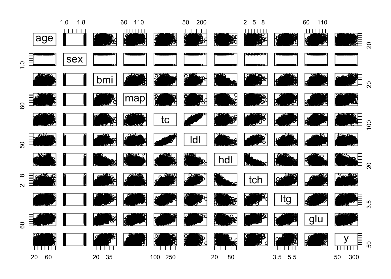
boxplot(diabetes) # always a good idea to check for gross outliers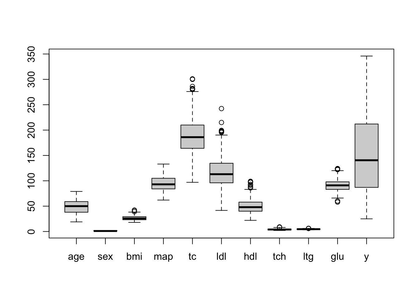
cor(diabetes)
Hmisc::describe(diabetes, digits=1) # summary of the diabetes data
skimr::skim(diabetes) # alternative summary method
Remark: Hmisc::describe returns Gmd, which is Gini’s mean difference, a robust measure of dispersion that is the mean absolute difference between any pairs of observations (see here for more information)
Try to find a couple of good models using the stepwise techniques discussed in lectures.
Backwards
M0 = lm(y ~ 1, data = diabetes)  # Null model
M1 = lm(y ~ ., data = diabetes)  # Full model
summary(M1)
##
## Call:
## lm(formula = y ~ ., data = diabetes)
##
## Residuals:
## Min 1Q Median 3Q Max
## -155.827 -38.536 -0.228 37.806 151.353
##
## Coefficients:
## Estimate Std. Error t value Pr(>|t|)
## (Intercept) -334.56714 67.45462 -4.960 1.02e-06 ***
## age -0.03636 0.21704 -0.168 0.867031
## sex -22.85965 5.83582 -3.917 0.000104 ***
## bmi 5.60296 0.71711 7.813 4.30e-14 ***
## map 1.11681 0.22524 4.958 1.02e-06 ***
## tc -1.09000 0.57333 -1.901 0.057948 .
## ldl 0.74645 0.53083 1.406 0.160390
## hdl 0.37200 0.78246 0.475 0.634723
## tch 6.53383 5.95864 1.097 0.273459
## ltg 68.48312 15.66972 4.370 1.56e-05 ***
## glu 0.28012 0.27331 1.025 0.305990
## ---
## Signif. codes: 0 '***' 0.001 '**' 0.01 '*' 0.05 '.' 0.1 ' ' 1
##
## Residual standard error: 54.15 on 431 degrees of freedom
## Multiple R-squared: 0.5177, Adjusted R-squared: 0.5066
## F-statistic: 46.27 on 10 and 431 DF, p-value: < 2.2e-16dim(diabetes)## [1] 442 11Try doing backward selection using AIC first, then using BIC. Do you get the same result?
Hint: Specify the option direction and k in the function step() correctly.
step.back.bic = step(M1, direction = "backward", trace = FALSE, k = log(442))
summary(step.back.bic)
##
## Call:
## lm(formula = y ~ sex + bmi + map + tc + ldl + ltg, data = diabetes)
##
## Residuals:
## Min 1Q Median 3Q Max
## -158.275 -39.476 -2.065 37.219 148.690
##
## Coefficients:
## Estimate Std. Error t value Pr(>|t|)
## (Intercept) -313.7666 25.3848 -12.360 < 2e-16 ***
## sex -21.5910 5.7056 -3.784 0.000176 ***
## bmi 5.7111 0.7073 8.075 6.69e-15 ***
## map 1.1266 0.2158 5.219 2.79e-07 ***
## tc -1.0429 0.2208 -4.724 3.12e-06 ***
## ldl 0.8433 0.2298 3.670 0.000272 ***
## ltg 73.3065 7.3083 10.031 < 2e-16 ***
## ---
## Signif. codes: 0 '***' 0.001 '**' 0.01 '*' 0.05 '.' 0.1 ' ' 1
##
## Residual standard error: 54.06 on 435 degrees of freedom
## Multiple R-squared: 0.5149, Adjusted R-squared: 0.5082
## F-statistic: 76.95 on 6 and 435 DF, p-value: < 2.2e-16step.back.aic = step(M1, direction = "backward", trace = FALSE, k = 2)
summary(step.back.aic)##
## Call:
## lm(formula = y ~ sex + bmi + map + tc + ldl + ltg, data = diabetes)
##
## Residuals:
## Min 1Q Median 3Q Max
## -158.275 -39.476 -2.065 37.219 148.690
##
## Coefficients:
## Estimate Std. Error t value Pr(>|t|)
## (Intercept) -313.7666 25.3848 -12.360 < 2e-16 ***
## sex -21.5910 5.7056 -3.784 0.000176 ***
## bmi 5.7111 0.7073 8.075 6.69e-15 ***
## map 1.1266 0.2158 5.219 2.79e-07 ***
## tc -1.0429 0.2208 -4.724 3.12e-06 ***
## ldl 0.8433 0.2298 3.670 0.000272 ***
## ltg 73.3065 7.3083 10.031 < 2e-16 ***
## ---
## Signif. codes: 0 '***' 0.001 '**' 0.01 '*' 0.05 '.' 0.1 ' ' 1
##
## Residual standard error: 54.06 on 435 degrees of freedom
## Multiple R-squared: 0.5149, Adjusted R-squared: 0.5082
## F-statistic: 76.95 on 6 and 435 DF, p-value: < 2.2e-16Forwards
Explore the forwards selection technique, which works very similarly to backwards selection, just set direction = "forward" in the step() function. When using direction = "forward" you need to sepecify a scope parameter: scope = list(lower = M0, upper = M1).
step.fwd.bic = step(M0, scope = list(lower = M0, upper = M1), direction = "forward",
                    trace = FALSE, k = log(442))
summary(step.fwd.bic)
##
## Call:
## lm(formula = y ~ bmi + ltg + map + tc + sex + ldl, data = diabetes)
##
## Residuals:
## Min 1Q Median 3Q Max
## -158.275 -39.476 -2.065 37.219 148.690
##
## Coefficients:
## Estimate Std. Error t value Pr(>|t|)
## (Intercept) -313.7666 25.3848 -12.360 < 2e-16 ***
## bmi 5.7111 0.7073 8.075 6.69e-15 ***
## ltg 73.3065 7.3083 10.031 < 2e-16 ***
## map 1.1266 0.2158 5.219 2.79e-07 ***
## tc -1.0429 0.2208 -4.724 3.12e-06 ***
## sex -21.5910 5.7056 -3.784 0.000176 ***
## ldl 0.8433 0.2298 3.670 0.000272 ***
## ---
## Signif. codes: 0 '***' 0.001 '**' 0.01 '*' 0.05 '.' 0.1 ' ' 1
##
## Residual standard error: 54.06 on 435 degrees of freedom
## Multiple R-squared: 0.5149, Adjusted R-squared: 0.5082
## F-statistic: 76.95 on 6 and 435 DF, p-value: < 2.2e-16step.fwd.aic = step(M0, scope = list(lower = M0, upper = M1), direction = "forward",
trace = FALSE, k = 2)
summary(step.fwd.aic)##
## Call:
## lm(formula = y ~ bmi + ltg + map + tc + sex + ldl, data = diabetes)
##
## Residuals:
## Min 1Q Median 3Q Max
## -158.275 -39.476 -2.065 37.219 148.690
##
## Coefficients:
## Estimate Std. Error t value Pr(>|t|)
## (Intercept) -313.7666 25.3848 -12.360 < 2e-16 ***
## bmi 5.7111 0.7073 8.075 6.69e-15 ***
## ltg 73.3065 7.3083 10.031 < 2e-16 ***
## map 1.1266 0.2158 5.219 2.79e-07 ***
## tc -1.0429 0.2208 -4.724 3.12e-06 ***
## sex -21.5910 5.7056 -3.784 0.000176 ***
## ldl 0.8433 0.2298 3.670 0.000272 ***
## ---
## Signif. codes: 0 '***' 0.001 '**' 0.01 '*' 0.05 '.' 0.1 ' ' 1
##
## Residual standard error: 54.06 on 435 degrees of freedom
## Multiple R-squared: 0.5149, Adjusted R-squared: 0.5082
## F-statistic: 76.95 on 6 and 435 DF, p-value: < 2.2e-16The add1 and drop1 command
Try using the add1() function. The general form is add1(fitted.model, test = "F", scope = M1).
add1(step.fwd.bic, test = "F", scope = M1)## Single term additions
##
## Model:
## y ~ bmi + ltg + map + tc + sex + ldl
## Df Sum of Sq RSS AIC F value Pr(>F)
## <none> 1271494 3534.3
## age 1 10.9 1271483 3536.3 0.0037 0.9515
## hdl 1 394.8 1271099 3536.1 0.1348 0.7137
## tch 1 3686.2 1267808 3535.0 1.2619 0.2619
## glu 1 3532.6 1267961 3535.0 1.2091 0.2721There is also the drop1() function, what does it return?
drop1(step.fwd.bic, test = "F")## Single term deletions
##
## Model:
## y ~ bmi + ltg + map + tc + sex + ldl
## Df Sum of Sq RSS AIC F value Pr(>F)
## <none> 1271494 3534.3
## bmi 1 190592 1462086 3594.0 65.205 6.687e-15 ***
## ltg 1 294092 1565586 3624.2 100.614 < 2.2e-16 ***
## map 1 79625 1351119 3559.1 27.241 2.787e-07 ***
## tc 1 65236 1336730 3554.4 22.318 3.123e-06 ***
## sex 1 41856 1313350 3546.6 14.320 0.0001758 ***
## ldl 1 39377 1310871 3545.7 13.472 0.0002723 ***
## ---
## Signif. codes: 0 '***' 0.001 '**' 0.01 '*' 0.05 '.' 0.1 ' ' 1Body fat
Your turn: explore with the body fat data set. Using the techniques outlined in the first lecture identify one (or more) models that help explain the body fat percentage of an individual.
data("bodyfat", package = "mplot")
# help("bodyfat", package = "mplot")
dim(bodyfat)
## [1] 128 15names(bodyfat)## [1] "Id" "Bodyfat" "Age" "Weight" "Height" "Neck"
## [7] "Chest" "Abdo" "Hip" "Thigh" "Knee" "Ankle"
## [13] "Bic" "Fore" "Wrist"bfat = bodyfat[,-1] # remove the ID columnfull.bf = lm(Bodyfat ~ ., data = bfat)
null.bf = lm(Bodyfat ~ 1, data = bfat)
step1 = step(full.bf, direction = "backward")## Start: AIC=373.2
## Bodyfat ~ Age + Weight + Height + Neck + Chest + Abdo + Hip +
## Thigh + Knee + Ankle + Bic + Fore + Wrist
##
## Df Sum of Sq RSS AIC
## - Ankle 1 0.15 1898.7 371.21
## - Age 1 0.76 1899.3 371.25
## - Knee 1 1.47 1900.1 371.29
## - Bic 1 1.59 1900.2 371.30
## - Wrist 1 2.08 1900.7 371.34
## - Thigh 1 4.24 1902.8 371.48
## - Chest 1 5.07 1903.7 371.54
## - Hip 1 8.03 1906.6 371.74
## - Height 1 10.80 1909.4 371.92
## - Weight 1 20.62 1919.2 372.58
## <none> 1898.6 373.20
## - Fore 1 38.19 1936.8 373.74
## - Neck 1 56.38 1955.0 374.94
## - Abdo 1 1088.97 2987.6 429.22
##
## Step: AIC=371.21
## Bodyfat ~ Age + Weight + Height + Neck + Chest + Abdo + Hip +
## Thigh + Knee + Bic + Fore + Wrist
##
## Df Sum of Sq RSS AIC
## - Age 1 0.84 1899.6 369.26
## - Bic 1 1.90 1900.6 369.33
## - Knee 1 1.92 1900.7 369.33
## - Wrist 1 2.64 1901.4 369.38
## - Thigh 1 4.15 1902.9 369.48
## - Chest 1 5.55 1904.3 369.58
## - Hip 1 7.93 1906.7 369.74
## - Height 1 11.90 1910.6 370.01
## - Weight 1 23.59 1922.3 370.79
## <none> 1898.7 371.21
## - Fore 1 38.15 1936.9 371.75
## - Neck 1 57.25 1956.0 373.01
## - Abdo 1 1125.31 3024.1 428.78
##
## Step: AIC=369.26
## Bodyfat ~ Weight + Height + Neck + Chest + Abdo + Hip + Thigh +
## Knee + Bic + Fore + Wrist
##
## Df Sum of Sq RSS AIC
## - Knee 1 1.33 1900.9 367.35
## - Bic 1 1.92 1901.5 367.39
## - Wrist 1 1.93 1901.5 367.39
## - Thigh 1 3.37 1903.0 367.49
## - Chest 1 6.39 1906.0 367.69
## - Hip 1 8.14 1907.7 367.81
## - Height 1 12.16 1911.7 368.08
## - Weight 1 27.13 1926.7 369.08
## <none> 1899.6 369.26
## - Fore 1 37.85 1937.4 369.79
## - Neck 1 56.57 1956.1 371.02
## - Abdo 1 1346.09 3245.7 435.83
##
## Step: AIC=367.35
## Bodyfat ~ Weight + Height + Neck + Chest + Abdo + Hip + Thigh +
## Bic + Fore + Wrist
##
## Df Sum of Sq RSS AIC
## - Bic 1 2.03 1902.9 365.49
## - Thigh 1 2.63 1903.5 365.53
## - Wrist 1 2.73 1903.6 365.53
## - Chest 1 7.05 1908.0 365.82
## - Hip 1 7.62 1908.5 365.86
## - Height 1 11.23 1912.1 366.11
## <none> 1900.9 367.35
## - Weight 1 30.51 1931.4 367.39
## - Fore 1 39.05 1940.0 367.95
## - Neck 1 55.47 1956.4 369.03
## - Abdo 1 1345.48 3246.4 433.86
##
## Step: AIC=365.49
## Bodyfat ~ Weight + Height + Neck + Chest + Abdo + Hip + Thigh +
## Fore + Wrist
##
## Df Sum of Sq RSS AIC
## - Wrist 1 2.79 1905.7 363.68
## - Thigh 1 4.63 1907.6 363.80
## - Hip 1 7.50 1910.4 363.99
## - Chest 1 7.55 1910.5 363.99
## - Height 1 10.21 1913.1 364.17
## - Weight 1 29.27 1932.2 365.44
## <none> 1902.9 365.49
## - Fore 1 50.40 1953.3 366.83
## - Neck 1 54.04 1957.0 367.07
## - Abdo 1 1353.15 3256.1 432.24
##
## Step: AIC=363.68
## Bodyfat ~ Weight + Height + Neck + Chest + Abdo + Hip + Thigh +
## Fore
##
## Df Sum of Sq RSS AIC
## - Thigh 1 7.00 1912.7 362.14
## - Hip 1 8.01 1913.7 362.21
## - Chest 1 9.29 1915.0 362.30
## - Height 1 13.86 1919.6 362.60
## <none> 1905.7 363.68
## - Weight 1 36.34 1942.1 364.09
## - Fore 1 50.12 1955.8 365.00
## - Neck 1 79.05 1984.8 366.88
## - Abdo 1 1372.77 3278.5 431.12
##
## Step: AIC=362.14
## Bodyfat ~ Weight + Height + Neck + Chest + Abdo + Hip + Fore
##
## Df Sum of Sq RSS AIC
## - Hip 1 4.42 1917.1 360.44
## - Chest 1 5.38 1918.1 360.50
## - Height 1 8.62 1921.3 360.72
## - Weight 1 29.49 1942.2 362.10
## <none> 1912.7 362.14
## - Fore 1 51.53 1964.3 363.55
## - Neck 1 80.80 1993.5 365.44
## - Abdo 1 1372.41 3285.1 429.38
##
## Step: AIC=360.44
## Bodyfat ~ Weight + Height + Neck + Chest + Abdo + Fore
##
## Df Sum of Sq RSS AIC
## - Chest 1 12.90 1930.0 359.30
## - Height 1 17.44 1934.6 359.60
## <none> 1917.1 360.44
## - Fore 1 59.51 1976.6 362.35
## - Neck 1 76.42 1993.6 363.44
## - Weight 1 117.40 2034.5 366.05
## - Abdo 1 1370.48 3287.6 427.47
##
## Step: AIC=359.3
## Bodyfat ~ Weight + Height + Neck + Abdo + Fore
##
## Df Sum of Sq RSS AIC
## - Height 1 9.06 1939.1 357.90
## <none> 1930.0 359.30
## - Fore 1 59.13 1989.2 361.16
## - Neck 1 74.35 2004.4 362.14
## - Weight 1 107.93 2038.0 364.26
## - Abdo 1 1679.52 3609.6 437.43
##
## Step: AIC=357.9
## Bodyfat ~ Weight + Neck + Abdo + Fore
##
## Df Sum of Sq RSS AIC
## <none> 1939.1 357.90
## - Fore 1 52.30 1991.4 359.30
## - Neck 1 85.21 2024.3 361.40
## - Weight 1 133.93 2073.0 364.45
## - Abdo 1 2283.87 4223.0 455.52step2 = step(null.bf, scope=list(lower=null.bf,upper=full.bf), direction = "forward")## Start: AIC=525.59
## Bodyfat ~ 1
##
## Df Sum of Sq RSS AIC
## + Abdo 1 5376.2 2274.9 372.34
## + Chest 1 4166.5 3484.7 426.93
## + Weight 1 3348.3 4302.9 453.92
## + Hip 1 3011.2 4640.0 463.58
## + Thigh 1 2089.3 5561.8 486.77
## + Bic 1 1848.4 5802.8 492.20
## + Knee 1 1819.1 5832.0 492.84
## + Neck 1 1652.8 5998.3 496.44
## + Wrist 1 1350.2 6300.9 502.74
## + Ankle 1 989.0 6662.2 509.88
## + Fore 1 886.5 6764.7 511.83
## + Age 1 495.1 7156.1 519.03
## + Height 1 175.3 7475.8 524.63
## <none> 7651.2 525.59
##
## Step: AIC=372.34
## Bodyfat ~ Abdo
##
## Df Sum of Sq RSS AIC
## + Weight 1 228.962 2046.0 360.76
## + Neck 1 191.968 2082.9 363.06
## + Hip 1 180.253 2094.7 363.78
## + Wrist 1 134.105 2140.8 366.56
## + Ankle 1 119.710 2155.2 367.42
## + Knee 1 113.440 2161.5 367.79
## + Thigh 1 94.488 2180.4 368.91
## + Height 1 64.441 2210.5 370.66
## + Bic 1 53.419 2221.5 371.30
## <none> 2274.9 372.34
## + Chest 1 27.282 2247.6 372.80
## + Age 1 20.550 2254.4 373.18
## + Fore 1 15.172 2259.8 373.49
##
## Step: AIC=360.76
## Bodyfat ~ Abdo + Weight
##
## Df Sum of Sq RSS AIC
## + Neck 1 54.563 1991.4 359.30
## + Wrist 1 33.470 2012.5 360.65
## <none> 2046.0 360.76
## + Fore 1 21.648 2024.3 361.40
## + Hip 1 10.725 2035.2 362.09
## + Height 1 9.781 2036.2 362.15
## + Ankle 1 3.584 2042.4 362.54
## + Chest 1 2.967 2043.0 362.58
## + Age 1 2.596 2043.4 362.60
## + Bic 1 2.257 2043.7 362.62
## + Knee 1 1.891 2044.1 362.65
## + Thigh 1 0.161 2045.8 362.75
##
## Step: AIC=359.3
## Bodyfat ~ Abdo + Weight + Neck
##
## Df Sum of Sq RSS AIC
## + Fore 1 52.296 1939.1 357.90
## <none> 1991.4 359.30
## + Hip 1 24.094 1967.3 359.75
## + Bic 1 9.256 1982.1 360.71
## + Chest 1 7.046 1984.3 360.85
## + Wrist 1 6.772 1984.6 360.87
## + Ankle 1 5.096 1986.3 360.98
## + Knee 1 3.707 1987.7 361.07
## + Height 1 2.231 1989.2 361.16
## + Thigh 1 0.423 1991.0 361.28
## + Age 1 0.010 1991.4 361.30
##
## Step: AIC=357.9
## Bodyfat ~ Abdo + Weight + Neck + Fore
##
## Df Sum of Sq RSS AIC
## <none> 1939.1 357.90
## + Hip 1 16.7889 1922.3 358.78
## + Height 1 9.0643 1930.0 359.30
## + Wrist 1 8.3637 1930.7 359.34
## + Ankle 1 7.4509 1931.7 359.40
## + Chest 1 4.5251 1934.6 359.60
## + Knee 1 1.4926 1937.6 359.80
## + Thigh 1 1.0270 1938.1 359.83
## + Bic 1 0.3077 1938.8 359.88
## + Age 1 0.2046 1938.9 359.88summary(step1)##
## Call:
## lm(formula = Bodyfat ~ Weight + Neck + Abdo + Fore, data = bfat)
##
## Residuals:
## Min 1Q Median 3Q Max
## -9.1637 -2.8476 0.0877 2.7522 8.3342
##
## Coefficients:
## Estimate Std. Error t value Pr(>|t|)
## (Intercept) -41.88325 8.30967 -5.040 1.62e-06 ***
## Weight -0.22932 0.07868 -2.915 0.00423 **
## Neck -0.61856 0.26606 -2.325 0.02172 *
## Abdo 0.98046 0.08146 12.036 < 2e-16 ***
## Fore 0.43409 0.23834 1.821 0.07099 .
## ---
## Signif. codes: 0 '***' 0.001 '**' 0.01 '*' 0.05 '.' 0.1 ' ' 1
##
## Residual standard error: 3.971 on 123 degrees of freedom
## Multiple R-squared: 0.7466, Adjusted R-squared: 0.7383
## F-statistic: 90.58 on 4 and 123 DF, p-value: < 2.2e-16summary(step2)##
## Call:
## lm(formula = Bodyfat ~ Abdo + Weight + Neck + Fore, data = bfat)
##
## Residuals:
## Min 1Q Median 3Q Max
## -9.1637 -2.8476 0.0877 2.7522 8.3342
##
## Coefficients:
## Estimate Std. Error t value Pr(>|t|)
## (Intercept) -41.88325 8.30967 -5.040 1.62e-06 ***
## Abdo 0.98046 0.08146 12.036 < 2e-16 ***
## Weight -0.22932 0.07868 -2.915 0.00423 **
## Neck -0.61856 0.26606 -2.325 0.02172 *
## Fore 0.43409 0.23834 1.821 0.07099 .
## ---
## Signif. codes: 0 '***' 0.001 '**' 0.01 '*' 0.05 '.' 0.1 ' ' 1
##
## Residual standard error: 3.971 on 123 degrees of freedom
## Multiple R-squared: 0.7466, Adjusted R-squared: 0.7383
## F-statistic: 90.58 on 4 and 123 DF, p-value: < 2.2e-16Both forward and backward stepwise select a model with Fore, Neck, Weight and Abdo. It does look to be substantially better than a simple linear regression of Bodyfat on Abdo (the best simple linear regression model).
slr.bf = lm(Bodyfat ~ Abdo, data = bfat)
summary(slr.bf)
##
## Call:
## lm(formula = Bodyfat ~ Abdo, data = bfat)
##
## Residuals:
## Min 1Q Median 3Q Max
## -10.3542 -2.9928 0.2191 2.4967 10.0106
##
## Coefficients:
## Estimate Std. Error t value Pr(>|t|)
## (Intercept) -43.19058 3.63431 -11.88 <2e-16 ***
## Abdo 0.67411 0.03907 17.26 <2e-16 ***
## ---
## Signif. codes: 0 '***' 0.001 '**' 0.01 '*' 0.05 '.' 0.1 ' ' 1
##
## Residual standard error: 4.249 on 126 degrees of freedom
## Multiple R-squared: 0.7027, Adjusted R-squared: 0.7003
## F-statistic: 297.8 on 1 and 126 DF, p-value: < 2.2e-16summary(slr.bf)$adj.r.squared## [1] 0.7003103summary(step1)$adj.r.squared## [1] 0.7383196AIC(slr.bf)## [1] 737.59AIC(step1)## [1] 723.1457anova(slr.bf,step1)## Analysis of Variance Table
##
## Model 1: Bodyfat ~ Abdo
## Model 2: Bodyfat ~ Weight + Neck + Abdo + Fore
## Res.Df RSS Df Sum of Sq F Pr(>F)
## 1 126 2274.9
## 2 123 1939.1 3 335.82 7.1005 0.0001936 ***
## ---
## Signif. codes: 0 '***' 0.001 '**' 0.01 '*' 0.05 '.' 0.1 ' ' 1Exhaustive searches
Crime data
data("UScrime", package = "MASS")
n = nrow(UScrime)
M0 = lm(y ~ 1, data=UScrime) # Null model
M1 = lm(y ~ ., data=UScrime) # Full model- Use the
lmSubsets()function from the lmSubsets package to obtain the 50 best models for each model size and use theplot()function to plot their RSS (and BIC) against model dimension.
library(lmSubsets)
rgsbst.out = lmSubsets(y ~ ., data = UScrime, nbest = 50,
                        nmax = NULL,
                        method = "exhaustive")
plot(rgsbst.out)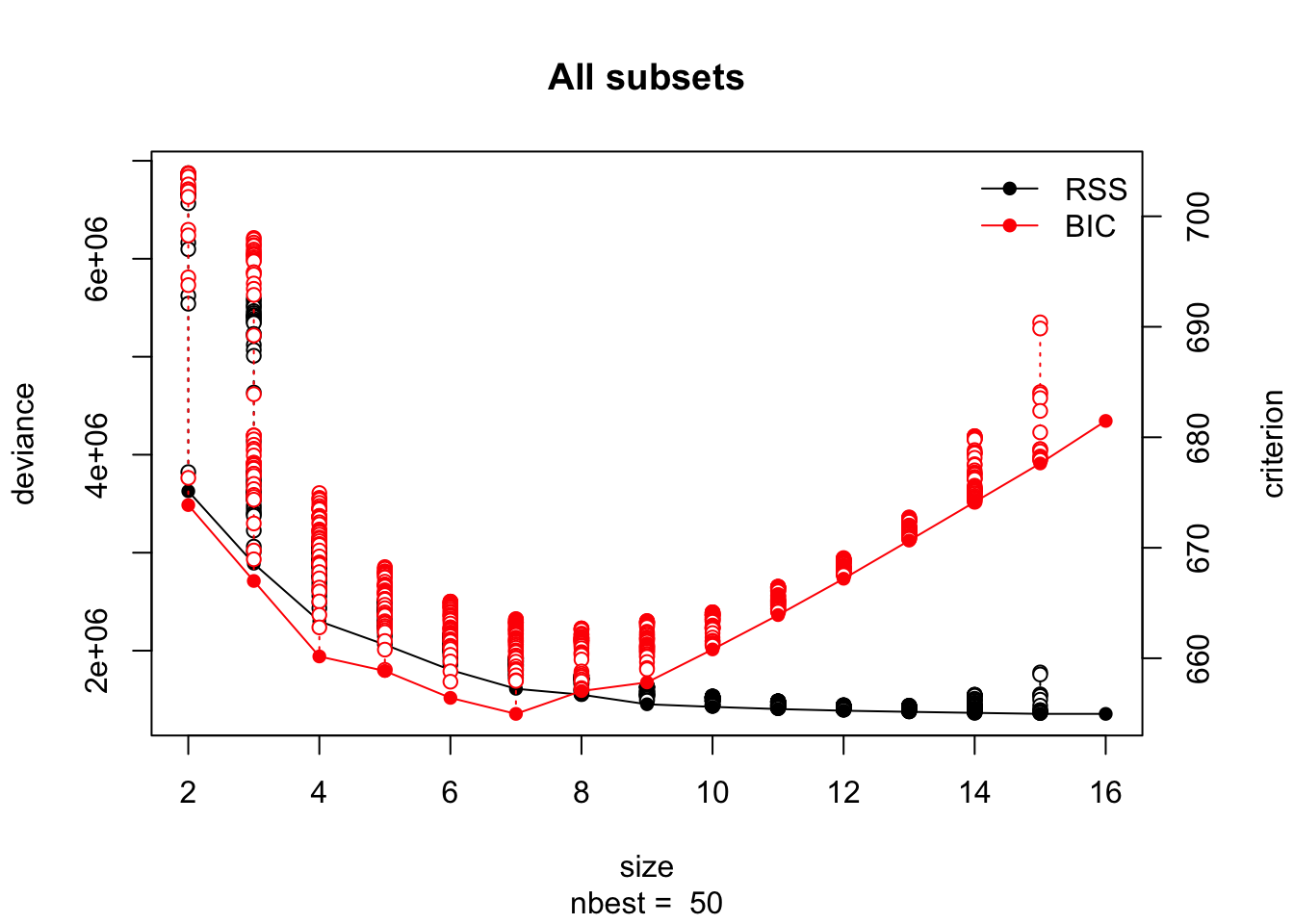
- Obtain and compare the best AIC and BIC models using the
lmSelect()function with forward and backwards stepwise procedures.
rgsbst.aic = lmSelect(y ~ ., data = UScrime, penalty = "AIC")
step.bwd.aic = step(M1, direction = "backward", trace = 0)
step.fwd.aic = step(M0, scope = list(upper = M1, lower = M0), direction = "forward", trace = 0)
rgsbst.bic = lmSelect(y ~ ., data = UScrime, penalty = "BIC")
step.bwd.bic = step(M1, k = log(n), direction = "backward", trace = 0)
step.fwd.bic = step(M0, k = log(n), scope = list(upper = M1, lower = M0), direction = "forward", trace = 0)
We can compare the models using the modelsummary package:
library(modelsummary)
msummary(list(`Exhaustive AIC` = refit(rgsbst.aic),
              `Step bwd AIC` = step.bwd.aic,
              `Step fwd AIC` = step.fwd.aic,
              `Exhaustive BIC` = refit(rgsbst.bic),
              `Step bwd BIC` = step.bwd.bic,
`Step fwd BIC` = step.fwd.bic))| Exhaustive AIC | Step bwd AIC | Step fwd AIC | Exhaustive BIC | Step bwd BIC | Step fwd BIC | |
|---|---|---|---|---|---|---|
| (Intercept) | -6426.101 | -6426.101 | -5040.505 | -5040.505 | -5040.505 | -5040.505 |
| (1194.611) | (1194.611) | (899.843) | (899.843) | (899.843) | (899.843) | |
| Ed | 18.012 | 18.012 | 19.647 | 19.647 | 19.647 | 19.647 |
| (5.275) | (5.275) | (4.475) | (4.475) | (4.475) | (4.475) | |
| Ineq | 6.133 | 6.133 | 6.765 | 6.765 | 6.765 | 6.765 |
| (1.396) | (1.396) | (1.394) | (1.394) | (1.394) | (1.394) | |
| M | 9.332 | 9.332 | 10.502 | 10.502 | 10.502 | 10.502 |
| (3.350) | (3.350) | (3.330) | (3.330) | (3.330) | (3.330) | |
| M.F | 2.234 | 2.234 | ||||
| (1.360) | (1.360) | |||||
| Po1 | 10.265 | 10.265 | 11.502 | 11.502 | 11.502 | 11.502 |
| (1.552) | (1.552) | (1.375) | (1.375) | (1.375) | (1.375) | |
| Prob | -3796.032 | -3796.032 | -3801.836 | -3801.836 | -3801.836 | -3801.836 |
| (1490.646) | (1490.646) | (1528.097) | (1528.097) | (1528.097) | (1528.097) | |
| U1 | -6.087 | -6.087 | ||||
| (3.339) | (3.339) | |||||
| U2 | 18.735 | 18.735 | 8.937 | 8.937 | 8.937 | 8.937 |
| (7.248) | (7.248) | (4.091) | (4.091) | (4.091) | (4.091) | |
| Num.Obs. | 47 | 47 | 47 | 47 | 47 | 47 |
| R2 | 0.789 | 0.789 | 0.766 | 0.766 | 0.766 | 0.766 |
| R2 Adj. | 0.744 | 0.744 | 0.731 | 0.731 | 0.731 | 0.731 |
| AIC | 639.3 | 639.3 | 640.2 | 640.2 | 640.2 | 640.2 |
| BIC | 657.8 | 657.8 | 655.0 | 655.0 | 655.0 | 655.0 |
| Log.Lik. | -309.658 | -309.658 | -312.083 | -312.083 | -312.083 | -312.083 |
They haven’t always selected identical models along the path. Exhaustive AIC and BIC select different models. All three BIC approaches selected the same model (forward, backward, exhaustive), but the forward AIC stepwise approach selected a different model to the exhaustive and backwards AIC approaches (interestingly the forward AIC model selected the same model as the BIC approaches).
Regularisation procedures
Ionosphere data
This is a data set from the UCI Machine Learning Repository. To make yourself familiar with the data, read an explanation.
We start by reading the data directly from the URL. There are many ways to read a file into R. For example:
- Because the entries are separated by a comma, we specify
sep=","in the functionread.table() - Use
read.csv() - Use the
read_csvfunction from the readr package which is faster thanread.csv() - Use the new vroom package, which automatically detects the separator (e.g. tab or comma), and is blindingly fast (vroom vroom).
url = "https://archive.ics.uci.edu/ml/machine-learning-databases/ionosphere/ionosphere.data"
dat = readr::read_csv(url, col_names = FALSE)
## Parsed with column specification:
## cols(
## .default = col_double(),
## X35 = col_character()
## )## See spec(...) for full column specifications.# install.packages("vroom")
# dat = vroom::vroom(url, col_names = FALSE)
# View(dat)
dim(dat)## [1] 351 35dat = dplyr::rename(dat, y = X35)
# names(dat)[35] = "y" # an alternative
dat$y = as.factor(dat$y)Look at the summary statistics for each variable and their scatterplot matrix. Show that column X2 is a vector of zeros and should therefore be omitted from the analysis.
# summary(dat) # output omitted
skimr::skim(dat)
boxplot(dat)
pairs(dat[, c(1:5, 35)])
table(dat$X2)
# Alternative methods:
# install.packages(Hmisc)
# Hmisc::describe(dat)
Delete the second column and make available a cleaned design matrix x with \(p=33\) columns and a response vector y of length \(n=351\), which is a factor with levels b and g.
x = as.matrix(dat[,-c(2,35)])
dim(x)
## [1] 351 33y = dat$y
is.factor(y)## [1] TRUEtable(y)## y
## b g
## 126 225Check the pairwise correlations in the design matrix and show that only one pair (the 12th and 14th column of x) of variables has an absolute Pearson correlation of more than 0.8.
round(cor(x),1)## X1 X3 X4 X5 X6 X7 X8 X9 X10 X11 X12 X13 X14
## X1 1.0 0.3 0.0 0.2 0.1 0.2 0.0 0.2 -0.1 0.0 0.1 0.1 0.2
## X3 0.3 1.0 0.1 0.5 0.0 0.4 0.0 0.5 0.0 0.3 0.2 0.2 0.2
## X4 0.0 0.1 1.0 0.0 -0.2 -0.1 0.3 -0.3 0.2 -0.2 0.3 -0.1 0.2
## X5 0.2 0.5 0.0 1.0 0.0 0.6 0.0 0.5 0.0 0.4 0.0 0.5 0.1
## X6 0.1 0.0 -0.2 0.0 1.0 0.0 0.3 -0.1 0.2 -0.3 0.2 -0.3 0.1
## X7 0.2 0.4 -0.1 0.6 0.0 1.0 -0.2 0.5 -0.1 0.4 0.0 0.6 0.1
## X8 0.0 0.0 0.3 0.0 0.3 -0.2 1.0 -0.3 0.4 -0.4 0.4 -0.4 0.3
## X9 0.2 0.5 -0.3 0.5 -0.1 0.5 -0.3 1.0 -0.3 0.7 -0.2 0.6 -0.1
## X10 -0.1 0.0 0.2 0.0 0.2 -0.1 0.4 -0.3 1.0 -0.3 0.4 -0.4 0.3
## X11 0.0 0.3 -0.2 0.4 -0.3 0.4 -0.4 0.7 -0.3 1.0 -0.2 0.6 -0.2
## X12 0.1 0.2 0.3 0.0 0.2 0.0 0.4 -0.2 0.4 -0.2 1.0 -0.2 0.4
## X13 0.1 0.2 -0.1 0.5 -0.3 0.6 -0.4 0.6 -0.4 0.6 -0.2 1.0 -0.1
## X14 0.2 0.2 0.2 0.1 0.1 0.1 0.3 -0.1 0.3 -0.2 0.4 -0.1 1.0
## X15 0.1 0.2 -0.3 0.4 -0.4 0.6 -0.4 0.6 -0.4 0.7 -0.2 0.8 -0.2
## X16 0.1 0.1 0.2 0.1 0.2 0.0 0.4 0.0 0.3 0.0 0.4 -0.2 0.2
## X17 0.1 0.2 -0.3 0.3 -0.3 0.4 -0.5 0.6 -0.4 0.7 -0.3 0.7 -0.3
## X18 0.1 0.2 -0.1 0.0 0.2 0.1 0.1 0.2 0.1 0.1 0.1 0.0 0.2
## X19 0.2 0.3 -0.3 0.2 -0.2 0.4 -0.4 0.7 -0.5 0.6 -0.4 0.6 -0.3
## X20 0.0 0.2 0.2 0.0 -0.1 0.2 0.1 0.1 0.0 0.1 0.1 0.2 0.4
## X21 0.2 0.1 -0.3 0.3 -0.1 0.6 -0.4 0.5 -0.4 0.5 -0.3 0.7 -0.3
## X22 -0.2 0.1 0.0 0.2 -0.1 0.2 -0.2 0.2 0.0 0.3 0.0 0.3 0.2
## X23 0.0 0.3 -0.1 0.5 -0.2 0.4 -0.3 0.4 -0.3 0.6 -0.4 0.5 -0.3
## X24 -0.1 0.0 0.2 0.1 -0.3 0.1 0.0 0.2 0.1 0.2 0.2 0.2 0.2
## X25 0.0 0.3 -0.1 0.2 -0.2 0.3 -0.2 0.4 -0.3 0.4 -0.2 0.4 -0.2
## X26 0.1 -0.1 -0.2 0.0 0.0 0.1 -0.1 0.1 0.0 0.1 -0.1 0.2 0.1
## X27 -0.2 0.1 0.0 0.1 -0.2 0.1 -0.3 0.2 -0.3 0.3 -0.2 0.3 -0.3
## X28 0.0 0.1 0.0 0.2 -0.1 0.1 0.1 0.1 0.1 0.2 0.1 0.1 0.1
## X29 0.1 0.3 0.0 0.3 0.0 0.3 -0.1 0.3 -0.1 0.4 -0.2 0.3 -0.2
## X30 -0.1 0.1 0.3 0.1 -0.2 0.0 0.1 0.0 0.0 0.1 0.1 0.1 0.1
## X31 0.2 0.2 -0.2 0.4 -0.1 0.4 -0.2 0.3 -0.2 0.3 -0.2 0.4 -0.1
## X32 -0.1 0.0 -0.1 0.0 0.3 0.0 0.2 -0.1 0.0 0.0 0.0 0.0 -0.1
## X33 0.2 0.3 -0.2 0.4 0.0 0.5 -0.2 0.3 -0.2 0.3 -0.2 0.5 -0.1
## X34 0.0 0.0 0.0 -0.1 0.2 -0.1 0.4 -0.1 0.1 -0.2 0.1 -0.1 0.1
## X15 X16 X17 X18 X19 X20 X21 X22 X23 X24 X25 X26 X27
## X1 0.1 0.1 0.1 0.1 0.2 0.0 0.2 -0.2 0.0 -0.1 0.0 0.1 -0.2
## X3 0.2 0.1 0.2 0.2 0.3 0.2 0.1 0.1 0.3 0.0 0.3 -0.1 0.1
## X4 -0.3 0.2 -0.3 -0.1 -0.3 0.2 -0.3 0.0 -0.1 0.2 -0.1 -0.2 0.0
## X5 0.4 0.1 0.3 0.0 0.2 0.0 0.3 0.2 0.5 0.1 0.2 0.0 0.1
## X6 -0.4 0.2 -0.3 0.2 -0.2 -0.1 -0.1 -0.1 -0.2 -0.3 -0.2 0.0 -0.2
## X7 0.6 0.0 0.4 0.1 0.4 0.2 0.6 0.2 0.4 0.1 0.3 0.1 0.1
## X8 -0.4 0.4 -0.5 0.1 -0.4 0.1 -0.4 -0.2 -0.3 0.0 -0.2 -0.1 -0.3
## X9 0.6 0.0 0.6 0.2 0.7 0.1 0.5 0.2 0.4 0.2 0.4 0.1 0.2
## X10 -0.4 0.3 -0.4 0.1 -0.5 0.0 -0.4 0.0 -0.3 0.1 -0.3 0.0 -0.3
## X11 0.7 0.0 0.7 0.1 0.6 0.1 0.5 0.3 0.6 0.2 0.4 0.1 0.3
## X12 -0.2 0.4 -0.3 0.1 -0.4 0.1 -0.3 0.0 -0.4 0.2 -0.2 -0.1 -0.2
## X13 0.8 -0.2 0.7 0.0 0.6 0.2 0.7 0.3 0.5 0.2 0.4 0.2 0.3
## X14 -0.2 0.2 -0.3 0.2 -0.3 0.4 -0.3 0.2 -0.3 0.2 -0.2 0.1 -0.3
## X15 1.0 -0.1 0.7 0.1 0.7 0.2 0.7 0.3 0.6 0.2 0.5 0.2 0.3
## X16 -0.1 1.0 -0.2 0.3 -0.3 0.3 -0.3 0.2 -0.2 0.2 -0.3 0.2 -0.3
## X17 0.7 -0.2 1.0 0.0 0.7 0.0 0.7 0.2 0.6 0.1 0.6 0.1 0.4
## X18 0.1 0.3 0.0 1.0 0.0 0.5 -0.1 0.4 -0.2 0.2 -0.2 0.4 -0.2
## X19 0.7 -0.3 0.7 0.0 1.0 0.0 0.7 0.1 0.6 0.1 0.5 0.2 0.4
## X20 0.2 0.3 0.0 0.5 0.0 1.0 -0.1 0.5 -0.1 0.3 -0.2 0.4 -0.2
## X21 0.7 -0.3 0.7 -0.1 0.7 -0.1 1.0 0.0 0.6 0.0 0.6 0.2 0.4
## X22 0.3 0.2 0.2 0.4 0.1 0.5 0.0 1.0 0.2 0.4 -0.1 0.4 0.0
## X23 0.6 -0.2 0.6 -0.2 0.6 -0.1 0.6 0.2 1.0 0.0 0.5 0.1 0.6
## X24 0.2 0.2 0.1 0.2 0.1 0.3 0.0 0.4 0.0 1.0 -0.1 0.4 0.0
## X25 0.5 -0.3 0.6 -0.2 0.5 -0.2 0.6 -0.1 0.5 -0.1 1.0 -0.1 0.5
## X26 0.2 0.2 0.1 0.4 0.2 0.4 0.2 0.4 0.1 0.4 -0.1 1.0 0.0
## X27 0.3 -0.3 0.4 -0.2 0.4 -0.2 0.4 0.0 0.6 0.0 0.5 0.0 1.0
## X28 0.2 0.2 0.2 0.3 0.2 0.3 0.1 0.4 0.2 0.4 0.2 0.4 0.1
## X29 0.4 -0.2 0.4 -0.1 0.5 -0.2 0.5 -0.1 0.5 -0.2 0.7 -0.1 0.5
## X30 0.1 0.1 0.1 0.1 0.1 0.4 0.1 0.3 0.2 0.4 0.0 0.3 0.2
## X31 0.4 -0.2 0.4 -0.2 0.4 -0.3 0.5 -0.1 0.5 -0.1 0.5 -0.2 0.4
## X32 0.0 0.1 0.0 0.3 0.1 0.1 0.1 0.2 0.2 0.1 0.1 0.3 0.2
## X33 0.5 -0.2 0.4 -0.1 0.4 -0.1 0.6 -0.1 0.5 -0.2 0.5 -0.1 0.5
## X34 -0.1 0.2 -0.1 0.1 0.0 0.2 0.0 0.1 0.0 0.1 0.1 0.2 0.1
## X28 X29 X30 X31 X32 X33 X34
## X1 0.0 0.1 -0.1 0.2 -0.1 0.2 0.0
## X3 0.1 0.3 0.1 0.2 0.0 0.3 0.0
## X4 0.0 0.0 0.3 -0.2 -0.1 -0.2 0.0
## X5 0.2 0.3 0.1 0.4 0.0 0.4 -0.1
## X6 -0.1 0.0 -0.2 -0.1 0.3 0.0 0.2
## X7 0.1 0.3 0.0 0.4 0.0 0.5 -0.1
## X8 0.1 -0.1 0.1 -0.2 0.2 -0.2 0.4
## X9 0.1 0.3 0.0 0.3 -0.1 0.3 -0.1
## X10 0.1 -0.1 0.0 -0.2 0.0 -0.2 0.1
## X11 0.2 0.4 0.1 0.3 0.0 0.3 -0.2
## X12 0.1 -0.2 0.1 -0.2 0.0 -0.2 0.1
## X13 0.1 0.3 0.1 0.4 0.0 0.5 -0.1
## X14 0.1 -0.2 0.1 -0.1 -0.1 -0.1 0.1
## X15 0.2 0.4 0.1 0.4 0.0 0.5 -0.1
## X16 0.2 -0.2 0.1 -0.2 0.1 -0.2 0.2
## X17 0.2 0.4 0.1 0.4 0.0 0.4 -0.1
## X18 0.3 -0.1 0.1 -0.2 0.3 -0.1 0.1
## X19 0.2 0.5 0.1 0.4 0.1 0.4 0.0
## X20 0.3 -0.2 0.4 -0.3 0.1 -0.1 0.2
## X21 0.1 0.5 0.1 0.5 0.1 0.6 0.0
## X22 0.4 -0.1 0.3 -0.1 0.2 -0.1 0.1
## X23 0.2 0.5 0.2 0.5 0.2 0.5 0.0
## X24 0.4 -0.2 0.4 -0.1 0.1 -0.2 0.1
## X25 0.2 0.7 0.0 0.5 0.1 0.5 0.1
## X26 0.4 -0.1 0.3 -0.2 0.3 -0.1 0.2
## X27 0.1 0.5 0.2 0.4 0.2 0.5 0.1
## X28 1.0 0.0 0.4 0.0 0.5 -0.1 0.4
## X29 0.0 1.0 0.0 0.6 0.1 0.6 0.1
## X30 0.4 0.0 1.0 -0.2 0.3 -0.2 0.4
## X31 0.0 0.6 -0.2 1.0 0.0 0.7 0.0
## X32 0.5 0.1 0.3 0.0 1.0 0.0 0.5
## X33 -0.1 0.6 -0.2 0.7 0.0 1.0 -0.1
## X34 0.4 0.1 0.4 0.0 0.5 -0.1 1.0# optional: visualise the correlation matrix
# install.packages("d3heatmap")
# d3heatmap::d3heatmap(cor(x))
cormat = cor(x)-diag(rep(1,33))
table(cormat>0.8)##
## FALSE TRUE
## 1087 2which(cormat>0.8)## [1] 377 441cormat[377]## [1] 0.8255584cor(x[,12],x[,14])## [1] 0.8255584# alternatively
# cordf = as.data.frame(as.table(cormat))
# subset(cordf, abs(Freq) > 0.8)
# or using the filter function from dplyr
# dplyr::filter(cordf, abs(Freq)>0.8)Logistic lasso regression
Fit a logistic lasso regression and comment on the lasso coefficient plot (showing \(\log(\lambda)\) on the x-axis and showing labels for the variables).
library(glmnet)## Warning: package 'glmnet' was built under R version 4.0.2lasso.fit = glmnet(x, y, family = "binomial")
plot(lasso.fit, xvar = "lambda", label = TRUE)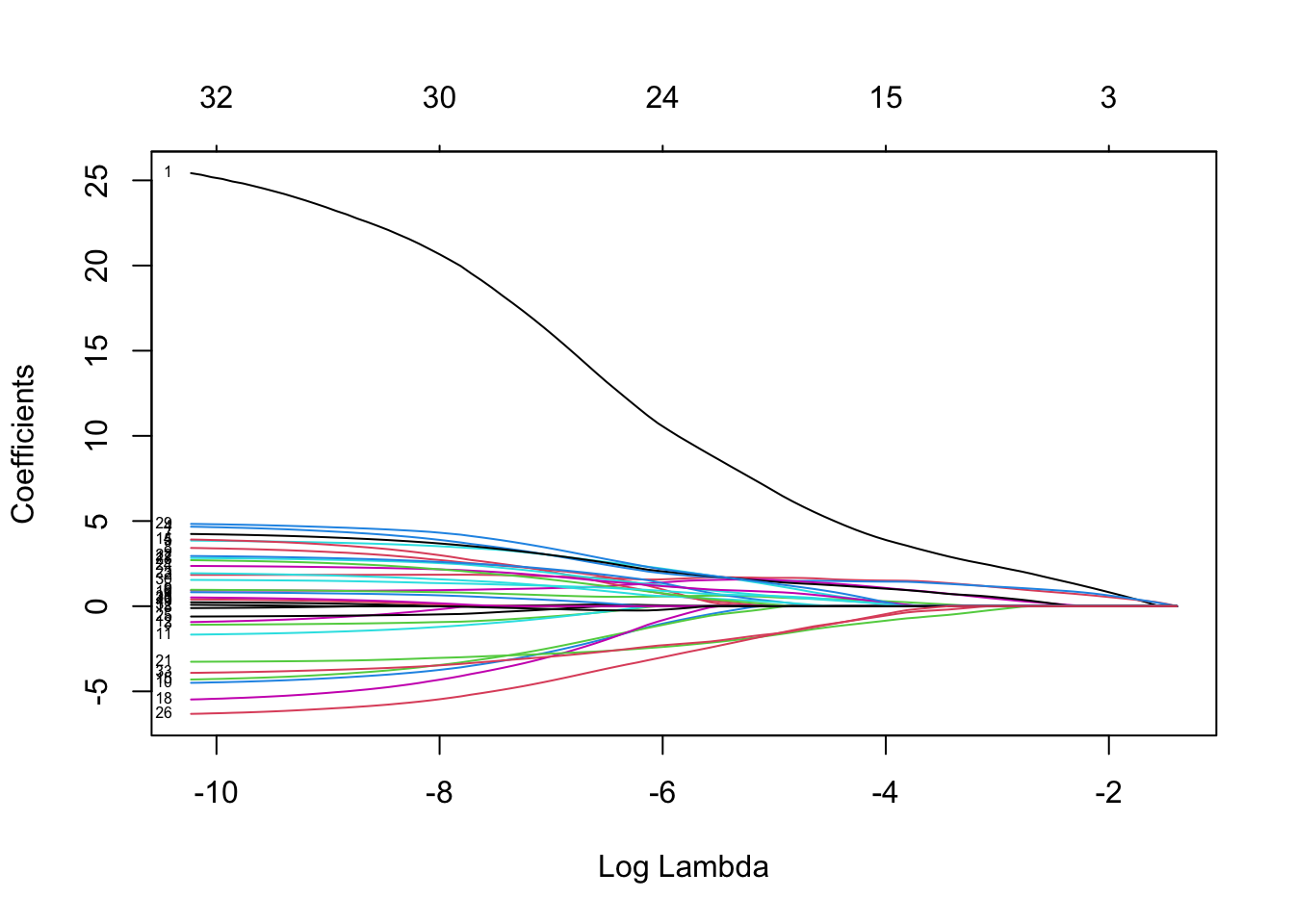
Choice of \(\lambda\) through AIC and BIC
Choose that \(\lambda\) value that gives smallest AIC and BIC for the models on the lasso path.
To calculate the \(-2\times\text{LogLik}\) for the models on the lasso path use the function deviance.glmnet (check help(deviance.glmnet)) and for calculating the number of non-zero regression parameters use the value df of the glmnet object.
Show also the corresponding regression coefficients.
length(lasso.fit$lambda)## [1] 96lasso.aic = deviance(lasso.fit) + 2*lasso.fit$df
lasso.bic = deviance(lasso.fit) + log(351)*lasso.fit$df
which.min(lasso.aic)## [1] 64which.min(lasso.bic)## [1] 37log(lasso.fit$lambda[64])## [1] -7.251293log(lasso.fit$lambda[37])## [1] -4.739382ic_coeffs = coef(lasso.fit)[,c(37,64)]
ic_coeffs## 34 x 2 sparse Matrix of class "dgCMatrix"
## s36 s63
## (Intercept) -7.63804244 -19.97760594
## X1 5.83649771 17.33128212
## X3 1.65355461 1.79013288
## X4 . -0.71473590
## X5 1.48511903 3.24988608
## X6 0.92605010 3.17590149
## X7 1.43732303 1.02380148
## X8 1.32579242 3.20339882
## X9 . 2.28104503
## X10 0.45782632 0.68954585
## X11 . -2.99786770
## X12 . -0.83889824
## X13 . .
## X14 . 0.03278883
## X15 . 2.30522823
## X16 . -2.74363799
## X17 . 0.43751730
## X18 0.45803345 2.13217256
## X19 . -3.35870761
## X20 . .
## X21 . .
## X22 -1.43984206 -2.85916411
## X23 0.08460504 2.31187561
## X24 0.12849989 1.30783045
## X25 0.72605376 1.89735684
## X26 . -0.27175033
## X27 -1.29590306 -4.69533343
## X28 . .
## X29 . 1.73637193
## X30 1.09798231 3.67431267
## X31 0.52476560 1.23671045
## X32 . .
## X33 . -0.12089348
## X34 -1.34765320 -3.09040097# count the number of non-zero coefficients in each column
diff(ic_coeffs@p)## [1] 17 29# help("CsparseMatrix-class")We can see that the BIC approach picks a much smaller model than the AIC approach.
Choice of \(\lambda\) through CV
Use cv.glmnet() to get the two default choices lambda.min and lambda.1se for the lasso tuning parameter \(\lambda\) when the classification error is minimised. Calculate these two values on the log-scale as well to relate to the above lasso coefficient plot.
set.seed(1)
lasso.cv = cv.glmnet(x, y, family = "binomial", type.measure = "class")
c(lasso.cv$lambda.min,lasso.cv$lambda.1se)
## [1] 0.0005365265 0.0115591136round(log(c(lasso.cv$lambda.min,lasso.cv$lambda.1se)),2)## [1] -7.53 -4.46plot(lasso.cv)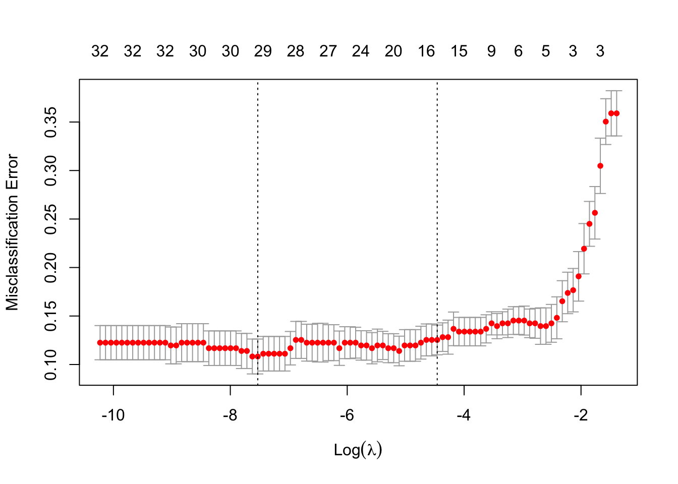
Explore how sensitive the lambda.1se value is to different choices of \(k\) in the \(k\)-fold CV (changing the default option nfolds=10) as well as to different choices of the random seed. (For each lambda value, the SE is estimated from the prediction errors over each of the \(k\) CV folds. The 1SE lambda value corresponds to the largest tuning parameter that has an estimated mean prediction error within the 1SE bounds of the lambda value that minimised the prediction error. For further details see Fig 2, as well as here and here.)
set.seed(2)
lasso.cv = cv.glmnet(x, y, family = "binomial", type.measure = "class", nfolds = 10)
round(log(lasso.cv$lambda.1se),2)
## [1] -4.27lasso.cv = cv.glmnet(x, y, family = "binomial", type.measure = "class", nfolds = 5)
round(log(lasso.cv$lambda.1se),2)## [1] -4.55lasso.cv = cv.glmnet(x, y, family = "binomial", type.measure = "class", nfolds = 3)
round(log(lasso.cv$lambda.1se),2)## [1] -2.69set.seed(3)
lasso.cv = cv.glmnet(x, y, family = "binomial", type.measure = "class", nfolds = 10)
round(log(lasso.cv$lambda.1se),2)## [1] -4.27lasso.cv = cv.glmnet(x, y, family = "binomial", type.measure = "class", nfolds = 5)
round(log(lasso.cv$lambda.1se),2)## [1] -2.51lasso.cv = cv.glmnet(x, y, family = "binomial", type.measure = "class", nfolds = 3)
round(log(lasso.cv$lambda.1se),2)## [1] -2.32# we could take a more organised approach to assess the variability:
set.seed(2)
nreps = 25
lse_nfolds10 = lse_nfolds5 = lse_nfolds3 = rep(NA,nreps)
for(i in 1:nreps){
lasso.cv = cv.glmnet(x, y, family="binomial", type.measure="class",nfolds=10)
lse_nfolds10[i] = log(lasso.cv$lambda.1se)
lasso.cv = cv.glmnet(x, y, family="binomial", type.measure="class",nfolds=5)
lse_nfolds5[i] = log(lasso.cv$lambda.1se)
lasso.cv = cv.glmnet(x, y, family="binomial", type.measure="class",nfolds=3)
lse_nfolds3[i] = log(lasso.cv$lambda.1se)
}
boxplot(lse_nfolds10,lse_nfolds5,lse_nfolds3,
names = c("nfolds=10","nfolds=5","nfolds=3"),
xlab = "log(Lambda)", horizontal = TRUE, las = 1)Marginality
In the lecture we briefly discussed the hierNet (pronounced “hair net”) package. Other packages that implement similar algorithms include:
- Regularization algorithm under marginality principle RAMP
- Learning Interactions via Hierarchical Group-Lasso Regularization glinternet. For a brief tutorial see here.
- A Convex Formulation for Modeling Interactions with Strong Heredity FAMILY
- sail: Sparse Additive Interaction Learning
These packages tend to be not particularly user friendly. Here we will explore RAMP and hierNet.
# install.packages("RAMP")
# install.packages("hierNet")
library(RAMP)
library(hierNet)
Using the same example from the lecture, we can compare the RAMP and heirNet results.
data("wallabies", package = "mplot")
X = subset(wallabies, select = c(-rw,-lat,-long))
y = wallabies$rw
Xy = as.data.frame(cbind(X, y))
Xm = X[, 1:5]  # main effects only
Xm = scale(Xm, center = TRUE, scale = TRUE)
# heirNet (from lectures)
fit = hierNet.logistic.path(Xm, y, diagonal=FALSE,
                            strong=TRUE)
set.seed(9)
fitcv=hierNet.cv(fit,Xm,y,trace=0)
fit.1se = hierNet.logistic(Xm, y, lam=fitcv$lamhat.1se,
                           diagonal = FALSE, strong = TRUE)
print(fit.1se)
# RAMP (equivalent RAMP code)
ramp = RAMP(Xm, y, family = "binomial", hier = "Strong")
ramp
Both approaches selet only one main effect, edible.
Diabetes
Your turn: Returning to the diabetes example, use both the RAMP and the hierNet package to determine a good model from the set of variables that includes all pairwise interactions.
data("diabetes", package="mplot")
X = scale(diabetes[,1:10], center = TRUE, scale = TRUE)
y = diabetes[,11]
ramp_db = RAMP(X, y, family = "gaussian", hier = "Strong")
ramp_db
## Important main effects: 2 3 4 7 9
## Coefficient estimates for main effects: -11.2 24.5 14.41 -14.11 23.1
## Important interaction effects: X3X4
## Intercept estimate: 148.9# names(ramp_db)
plot(ramp_db$cri.list ~ ramp_db$lambda, log = "x", ylab = "EBIC", xlab = "lambda")
# identify that minimum criterion value
which.min(ramp_db$cri.list)
## [1] 22# this is output as cri.loc
ramp_db$cri.loc## [1] 22# corresponding interactions:
ramp_db$interInd## [1] "X3X4"ramp_db$interInd.list[[ramp_db$cri.loc]]## [1] "X3X4"colnames(X)[c(3,4)]## [1] "bmi" "map"# corresponding main effects:
ramp_db$mainInd## [1] 2 3 4 7 9ramp_db$mainInd.list[[ramp_db$cri.loc]]## [1] 2 3 4 7 9colnames(X)[ramp_db$mainInd.list[[ramp_db$cri.loc]]]## [1] "sex" "bmi" "map" "hdl" "ltg"We can see that the selected model has sex, bmi, map, hdl and ltg as main effects with an interaction between bmi and map.
set.seed(1)
fit_db = hierNet.path(X, y, diagonal=FALSE, strong=TRUE)
fitcv_db = hierNet.cv(fit_db, X, y, trace=0, nfolds = 10)
fitcv_db$lamhat
fit_1se_db = hierNet(X, as.numeric(y),
                     lam = fitcv_db$lamhat.1se,
                     diagonal = FALSE, strong = TRUE)
fit_1se_db
colnames(X)[c(2,3,4,7,9,10)]
We get a slightly larger model out of the hierNet package, with the addition of the glu main effect and the interaction between glu and bmi. This may also depend on the seed and the number of folds selected as the CV method is inherently random.
References
- Efron B, Hastie T, Johnstone I and Tibshirani R (2004). Least angle regression. The Annals of Statistics 32(2): 407-499. doi:10.1214/009053604000000067
- Johnson RW (1996). Fitting Percentage of Body Fat to Simple Body Measurements. Journal of Statistics Education (4)1, http://www.amstat.org/publications/jse/v4n1/datasets.johnson.html