Lecture B

class: center, middle, inverse, title-slide

# Lecture B
## Exhaustive and non-exhaustive algorithms with resampling
### Samuel Müller and Garth Tarr

---

## Overview

B1. Cross validation

B2. .blue[The `mplot` package]
* .red[Artificial example]: *Information criteria can be blind*
* .blue[Variable inclusion plots]
* .blue[Model stability plots]
* .blue[Bootstraping the lasso]

B3. Subtractive stability measures

---
class: segue

# B1. Cross-validation for model selection

---

## Resampling procedures

- .orange[Cross-validation (CV)] and .red[bootstrapping] are the two most popular classes of .blue[resampling methods] in model building
- In model building, resampling is often used to
- assess the <span style="color:blue">stability</span> of a model
- infer on model parameters (tests, <span style="color:blue">confidence intervals</span>, point estimates, <span style="color:blue">bias</span>)
- measure .blue[prediction error]

---

## Cross-validation algorithms

- .orange[Cross-validation] schemes can be implemented in most statistical frameworks and for most estimation procedures
- The key principle of CV is to .blue[split the data] into a .blue[training set] and a .red[validation set] 
- .blue[Estimators] are .blue[built on the training set]
- .red[Validation set] is used .red[to] validate/.red[assess] the .red[performance] of the estimators, e.g. estimating their prediction risk 
- This training / validation splitting is repeated several times

---

## 10-fold cross validation

---

## Cross-validation algorithms

The most popular .orange[cross-validation schemes] are,

- .blue[Hold-out CV], based on a single split of the data
- <span style="color:red"> `$\color{red}{k}$`-fold CV</span>: the data is split into `$k$` subsamples. Each subsample is successively removed for validation, the remaining data being used for training
- .blue[Leave-one-out] (LOOCV) which corresponds to <span style="color:red"> `$n$`-fold CV</span>
- <span style="color:blue">Leave- `$q$`-out</span> every of the `$\binom{n}{q}$` possible subsets is removed for validation

---

## CV prediction error

- In `$k$`-fold CV the data is split into `$k$` subsamples (the `$k$` folds)
- Each subsample is successively removed for .red[validation], the remaining data being used for .blue[training]
- Thus, for each of the `$k$` folds `$f=1,\ldots,k$`,  `$\iota_f\subset\{1,\ldots,n\}$` denotes the `$n_f = |\iota_f|$` observations in the `$f$`th fold and we calculate
`$$\text{CV}_{(k)} = \frac{1}{k} \sum_{f=1}^k \text{MSE}_f = \frac{1}{k}\sum_{f=1}^k \frac{1}{n_f}\sum_{i\in \iota_f} [y_i - \hat y_{\alpha i}(-\iota_f)]^2$$`
- Similarly, for estimating classification errors

---

## Choice of `$k$` affects the quality of the CV error

- If `$\color{blue}{k=2}$`: split-sample CV - CV error estimates .blue[biased] upwards because only half the data used in the training samples
- If `$\color{red}{k=n}$`: LOOCV - CV estimates have .red[high variance] because in the above equation a total of `$n$` positively correlated quantities are averaged;
- .blue[Standard choices] are `$\color{blue}{k=10}$` (default in `cv.glmnet` through option `nfolds=10`) or `$k=5$`: This balances bias and variance 
- The `$k$` partly overlapping training sets can be used to learn more about the stability of selected models

---
class: segue

# Case study: selecting `$\lambda$` for Lasso

---

## How to best choose `$\lambda$`?

- Many options!
- .blue[Use information criteria along the lasso], ridge, or elastic-net .blue[path]
- Use cross-validation
- as an alternative to `lambda.min` often `lambda.1se` does give better performance in terms of prediction
- `lambda.1se` is the largest `$\lambda$` at which the MSE is within one standard error of the minimal MSE (at `lambda.min`)

---
class: eg

### Diabetes example

```r
data("diabetes", package = "lars")
library("glmnet")
x = diabetes$x2 # includes squares and interactions
y = diabetes$y
lasso.fit = glmnet(x, y)
length(lasso.fit$lambda)
```

```
## [1] 100
```

```r
lasso.predict = predict(lasso.fit, newx = x)
dim(lasso.predict)
```

```
## [1] 442 100
```

---
class: eg

### Diabetes example: AIC to select `$\lambda$`

```r
lasso.aic = rep(0, 100)
sigma.hat = summary(lm(y ~ x))$s
for (m in 1:100) {
  yhat = lasso.predict[, m]
  k = lasso.fit$df[m]
  lasso.aic[m] = sum((y - yhat)^2)/(sigma.hat^2) + 2*k
}
which.min(lasso.aic)
```

```
## [1] 32
```

```r
lasso.fit$lambda[32]
```

```
## [1] 2.524812
```

---
class: eg

### Diabetes example: CV to select `$\lambda$`

```r
set.seed(2020)
lasso.cv = cv.glmnet(x, y)
plot(lasso.cv)
abline(h = min(lasso.cv$cvm) + lasso.cv$cvsd[which.min(lasso.cv$cvm)], 
       col = "blue")
```

```r
lasso.cv$lambda.1se
```

```
## [1] 5.314486
```

---
class: eg

### Diabetes example:

Predictors selected by .bold[.blue[AIC]]:

```r
aic_betas = glmnet(x, y, lambda = lasso.fit$lambda[32])$beta
as.matrix(aic_betas)[as.matrix(aic_betas)>0, ]
```

```
##        bmi        map        ltg        glu      age^2      bmi^2 
## 500.775931 262.976223 469.918325  25.416346  17.558198  42.899478 
##      glu^2    age:sex    age:map    age:ltg    age:glu    sex:map 
##  76.518096 115.463280  30.647942  12.662471   9.365541   7.745166 
##    bmi:map 
##  90.571069
```

Predictors selected by .bold[.red[CV]]:

```r
cv_betas = glmnet(x, y, lambda = lasso.cv$lambda.1se)$beta
as.matrix(cv_betas)[as.matrix(cv_betas)>0,]
```

```
##        bmi        map        ltg      bmi^2      glu^2    age:sex 
## 502.887614 205.892655 453.531965  17.266008  39.776736  60.581213 
##    age:map    age:glu    bmi:map 
##  14.945884   7.108415  59.023875
```

---
class: eg

### Diabetes example

We can choose between the two competing models using **cross validation**.

```r
library(caret)
control <- trainControl(method = "cv", number = 10)
dat <- cbind(y, x)
aic_cv <- train(y ~ bmi + map + ltg + glu + `age^2` + `bmi^2` + 
                  `glu^2` + `age:sex` + `age:map` + `age:ltg` + 
                  `age:glu` + `sex:map` + `bmi:map`,
                method = "lm", data = dat, trControl = control)
cv_cv <- train(y ~ bmi + map + ltg + `bmi^2` + `glu^2` + 
                 `age:sex` + `age:map` + `age:glu` + `bmi:map`,
               method = "lm", data = dat, trControl = control)
results <- resamples(list(AIC = aic_cv, CV = cv_cv))
ggplot(results) + theme_classic(base_size = 18) +
  labs(x = "MAE")
```

---
class: segue

# B2. The mplot package

---

## Installing the mplot package

```r
# install.packages("devtools")
# devtools::install_github("garthtarr/mplot")
install.packages("mplot")
library(mplot)
```

Website: http://garthtarr.github.io/mplot

### Main functions

* `af()` for the adaptive fence for `lm()` and `glm()`
* `vis()` for variable importance plots and model stability plots for `lm()` and `glm()`
* `bglmnet()` for bootstrapping `glmnet()` and variable importance and model stability plots
* `mplot()` for an interactive shiny interface

.footnote[
Tarr, Müller, and Welsh (2018)
]

---

## Motivation – Recall Anscombe’s quartet

---

## Datasaurus

```r
library(datasauRus)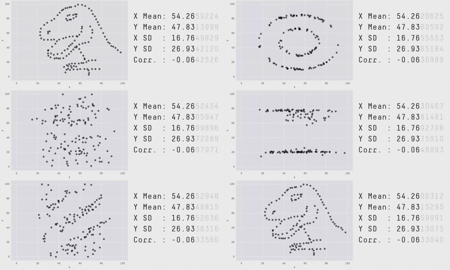
```

![](imgs/DinoSequentialSmaller.gif)

.footnote[
Matejka J and Fitzmaurice G (2017). [Same Stats, Different Graphs: Generating Datasets with Varied Appearance and Identical Statistics through Simulated Annealing.](https://www.autodeskresearch.com/publications/samestats) Autodesk Research, Toronto Ontario Canada. DOI: 10.1145/3025453.3025912 
]

---

## See also

![](imgs/boxplots.gif)

![](imgs/BoxViolinSmaller.gif)

---

## Graphical tools for model selection

* .red[Underused!]
* .blue[Fence] and its variants (series of papers by Jiang et al, starting with Jiang, Rao, Gu, and Nguyen (2008)) 
* .blue[Stability selection] Meinshausen and Bühlmann (2010)
* .blue[Model selection curves] Müller and Welsh (2010)
* .blue[Variable inclusion plots] Müller and Welsh (2010) and Murray, Heritier, and Müller (2013)
* .red[Variable selection with `mplot`] (this lecture)

---
class: segue

# Artificial example

---
class: eg

## Artificial example: Correlations

---
class: eg

## Artificial example: Full model

.scroll-output[

```r
library(mplot)
lm.art = lm(y ~ ., data = artificialeg)
summary(lm.art)
```

```
## 
## Call:
## lm(formula = y ~ ., data = artificialeg)
## 
## Residuals:
##     Min      1Q  Median      3Q     Max 
## -4.7254 -1.2126  0.2456  1.3446  3.4808 
## 
## Coefficients:
##             Estimate Std. Error t value Pr(>|t|)
## (Intercept)  -0.1002     0.3268  -0.307    0.761
## x1            0.6403     0.6924   0.925    0.361
## x2            0.2574     0.6176   0.417    0.679
## x3           -0.5105     1.2391  -0.412    0.683
## x4           -0.2978     0.2515  -1.184    0.243
## x5            0.3551     0.5982   0.594    0.556
## x6           -0.5428     0.9612  -0.565    0.575
## x7           -0.4280     0.6308  -0.678    0.501
## x8            0.1503     0.6175   0.243    0.809
## x9            0.3997     0.6379   0.627    0.535
## 
## Residual standard error: 2.023 on 40 degrees of freedom
## Multiple R-squared:  0.7508,	Adjusted R-squared:  0.6947 
## F-statistic: 13.39 on 9 and 40 DF,  p-value: 1.476e-09
```
]

---
class: eg

## Artificial example: Final model

.scroll-output[

```r
step(lm.art)
```

```
## Start:  AIC=79.3
## y ~ x1 + x2 + x3 + x4 + x5 + x6 + x7 + x8 + x9
## 
##        Df Sum of Sq    RSS    AIC
## - x8    1    0.2423 163.94 77.374
## - x3    1    0.6946 164.39 77.512
## - x2    1    0.7107 164.41 77.517
## - x6    1    1.3051 165.00 77.698
## - x5    1    1.4425 165.14 77.739
## - x9    1    1.6065 165.31 77.789
## - x7    1    1.8835 165.58 77.873
## - x1    1    3.4999 167.20 78.358
## - x4    1    5.7367 169.44 79.023
## <none>              163.70 79.301
## 
## Step:  AIC=77.37
## y ~ x1 + x2 + x3 + x4 + x5 + x6 + x7 + x9
## 
##        Df Sum of Sq    RSS     AIC
## <none>              163.94  77.374
## - x2    1    20.359 184.30  81.227
## - x5    1    25.966 189.91  82.726
## - x9    1    33.607 197.55  84.698
## - x4    1    34.504 198.45  84.925
## - x7    1    62.097 226.04  91.434
## - x1    1    68.253 232.19  92.778
## - x3    1    71.301 235.24  93.430
## - x6    1   107.873 271.81 100.655
```

```
## 
## Call:
## lm(formula = y ~ x1 + x2 + x3 + x4 + x5 + x6 + x7 + x9, data = artificialeg)
## 
## Coefficients:
## (Intercept)           x1           x2           x3           x4  
##     -0.1143       0.8019       0.4011      -0.8083      -0.3514  
##          x5           x6           x7           x9  
##      0.4927      -0.7738      -0.5772       0.5478
```
]

---
class: eg

## Artificial example: Final model

.scroll-output[

```r
lm.fin = lm(y ~ . - x8, data = artificialeg)
summary(lm.fin)
```

```
## 
## Call:
## lm(formula = y ~ . - x8, data = artificialeg)
## 
## Residuals:
##     Min      1Q  Median      3Q     Max 
## -4.6881 -1.2352  0.2787  1.4102  3.5420 
## 
## Coefficients:
##             Estimate Std. Error t value Pr(>|t|)    
## (Intercept)  -0.1143     0.3179  -0.360 0.720952    
## x1            0.8019     0.1941   4.132 0.000173 ***
## x2            0.4011     0.1778   2.256 0.029438 *  
## x3           -0.8083     0.1914  -4.223 0.000131 ***
## x4           -0.3514     0.1196  -2.938 0.005408 ** 
## x5            0.4927     0.1933   2.548 0.014667 *  
## x6           -0.7738     0.1490  -5.194    6e-06 ***
## x7           -0.5772     0.1465  -3.941 0.000309 ***
## x9            0.5478     0.1890   2.899 0.005987 ** 
## ---
## Signif. codes:  0 '***' 0.001 '**' 0.01 '*' 0.05 '.' 0.1 ' ' 1
## 
## Residual standard error: 2 on 41 degrees of freedom
## Multiple R-squared:  0.7504,	Adjusted R-squared:  0.7017 
## F-statistic: 15.41 on 8 and 41 DF,  p-value: 3.692e-10
```
]

---
class: eg

## Artificial example: Data generating model

The .red[true data generating model] is: `$\color{red}{y}  = 0.6\,\color{red}{x_8} + \color{red}{\varepsilon}$`.

```r
art.true = lm(y ~ x8, data = artificialeg)
summary(art.true)
```

```
## 
## Call:
## lm(formula = y ~ x8, data = artificialeg)
## 
## Residuals:
##     Min      1Q  Median      3Q     Max 
## -5.6013 -1.2985  0.1303  1.4605  3.8056 
## 
## Coefficients:
##             Estimate Std. Error t value Pr(>|t|)    
## (Intercept)  0.03235    0.29458    0.11    0.913    
## x8           0.54928    0.05264   10.43 6.18e-14 ***
## ---
## Signif. codes:  0 '***' 0.001 '**' 0.01 '*' 0.05 '.' 0.1 ' ' 1
## 
## Residual standard error: 2.046 on 48 degrees of freedom
## Multiple R-squared:  0.694,	Adjusted R-squared:  0.6877 
## F-statistic: 108.9 on 1 and 48 DF,  p-value: 6.18e-14
```

---
class: segue

# Information criteria can be blind

.blockquote[
Use resampling and graphs to **see** more!
]

---

## Bootstrapping regression models

.blockquote[
The **bootstrap** is a resampling strategy to generate `$B$` training sets
]

<br>

### Popular implementations

- **Paired bootstrap**: samples (with replacement) rows of `$[\boldsymbol{y},\boldsymbol{X}]$`

- .blue[**Weighted bootstrap**] (used in `vis()` and `bglmnet()`): mimics the paired bootstrap by keeping `$[\boldsymbol{y},\boldsymbol{X}]$` as is but weighs each observation (row) through using a weights vector, where the weights are sampled from a distribution with expectation 1 (e.g. exponential).

- .blue[**Parametric bootstrap**] (used in `af()`): estimate the (parametric) distribution of `$\boldsymbol{y}$` (or `$\boldsymbol{\varepsilon}$`) and draw new observations from it

- **Residual bootstrap**: baseline model + bootstrapped error
---

## Stability

- In practice it is important that selected models are stable

.blockquote[
**Key idea**: small changes should have small effects
]

- Example: Information criterion is *unstable* when `$\hat{\alpha}(\lambda)$` is selected with dimension `$p_{\hat{\alpha}(\lambda)}$` but, for some small `$\delta>0$`, `$\hat{\alpha}(\lambda+\delta)$` selected with `$p_{\hat{\alpha}(\lambda+\delta)} < p_{\hat{\alpha}(\lambda)}$`
- Investigate model selection criterion in a neighborhood of `$\lambda$`

---

## Obtaining stability information

.blockquote[
**Use resampling**: repeatedly calculate how well (the best) model(s) perform given `$\lambda$`, summarise performance with statistics and graphs
]

<br>

### We will do the following:

* Investigate model detectability as a function of `$\lambda$` 
* Estimate probability that model `$\alpha\in\mathcal{A}$` is optimal at `$\lambda$`
* Estimate best model(s) within each size/dimension
* Show model selection curves also for models that are never optimal

---
class: segue

# Variable inclusion plots

---

## Variable inclusion plots

.blockquote[
**Aim**: To visualise inclusion probabilities as a function of the penalty multiplier `$\lambda \in [0,2\log(n)]$`
]

### Procedure

1. Calculate (weighted) .red[bootstrap samples]  `$\color{red}{b}=1,\ldots,B$`.
2. For each .red[bootstrap sample], at each `$\color{blue}{\lambda}$` .blue[value], find `$\hat{\alpha}_{\color{blue}{\lambda}}^{(\color{red}{b})}\in\mathcal{A}$` as the model with smallest `$\text{GIC}(\alpha;\color{blue}{\lambda}) = -2\times \text{LogLik}(\alpha)+\color{blue}{\lambda} p_\alpha$`.
3. The **inclusion probability** for variable `$x_j$` is estimated as `$\frac{1}{B}\sum_{\color{red}{b}=1}^B 1\{j\in \hat{\alpha}_{\color{blue}{\lambda}}^{(\color{red}{b})}\}$`.

.blockquote[
The **inclusion probability** for variable `$x_j$` is the proportion of times variable `$x_j$` is in the best model
]

.footnote[
- Müller and Welsh (2010) for linear regression models 
- Murray, Heritier, and Müller (2013) for generalised linear models
]

---
class: eg

## Artificial example: VIP

```r
library(mplot)
vis.art = vis(lm.art)
plot(vis.art, which = "vip", interactive = TRUE)
```

---
class: segue

# Model stability plots

---
class: eg

## Artificial example: Loss against size

```r
plot(vis.art, which="lvk", interactive = TRUE)
```

---
class: eg

## Artificial example: Loss against size

```r
plot(vis.art, which = "lvk", highlight = "x6", interactive = TRUE)
```

---

## Model stability plots

.blockquote[
**Aim**: To add value to the loss against size plots by choosing a symbol size proportional to a measure of stability
]

<br>

### Procedure

1. Calculate (weighted) bootstrap samples `$b=1,\ldots,B$`
2. For each bootstrap sample, identify the *best* model at each dimension
3. Add this information to the loss against size plot using model identifiers that are proportional to the frequency with which a model was identified as being *best* at each model size

.footnote[
Murray, Heritier, and Müller (2013) for generalised linear models 
]

---
class: eg

## Artificial example: Model stability plot

```r
plot(vis.art, which = "boot", interactive = FALSE)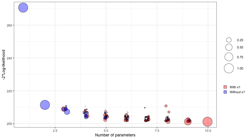
```
![](lecB_files/figure-html/unnamed-chunk-14-1.png)

---

## Artificial example: Model stability plot

```r
plot(vis.art, which = "boot", interactive = TRUE)
```

---
class: segue

# Bootstrapping the lasso

---
class: eg

## Artificial example: Lasso

```r
library(lars)
x = as.matrix(subset(artificialeg, select = -y))
y = as.matrix(subset(artificialeg, select = y))
art.lars=lars(x, y)
plot(art.lars, xvar = "step", breaks = FALSE, lwd = 2, cex.lab = 1.4)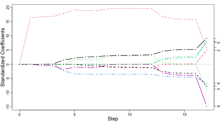
```

![](lecB_files/figure-html/lars1-1.png)

---
class: eg

## Artificial example: Lasso

```r
plot(art.lars, xvar = "step", plottype = "Cp", lwd = 2, cex.lab = 1.4)
```

![](lecB_files/figure-html/lars2-1.png)

---
class: eg

## Artificial example: Lasso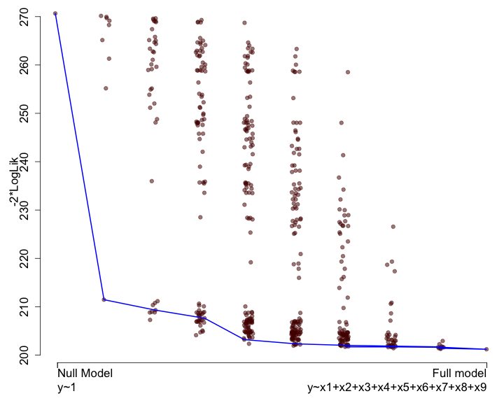

![](lecB_files/figure-html/lassoplot1-1.png)

---
class: eg

## Artificial example: Lasso (zoomed)

![](lecB_files/figure-html/lassoplot5-1.png)

---
class: eg

## Bootstrapping the lasso

```r
bgn.art = bglmnet(lm.art, lambda = seq(0.05, 2.75, 0.1))
plot(bgn.art, which = "boot", interactive = TRUE)
```

---
class: eg

## Bootstrapping the lasso

```r
bgn.art = bglmnet(lm.art)
plot(bgn.art, which = "vip", interactive = TRUE)
```

---
class: segue

# B3. Subtractive stability measures

# `$\hat{Q}(M) = s - \sum_{j\in M}s_j$`

---

## Stability measures

- Use .red[resampling], say `$B$` resamples (100, 1000 or more)
- Consider .blue[baseline models] (e.g. all models on a solution path), say `$K$` such models
- Learn from an array of `$K\times p\times B$` regression coefficients
- Calculate for each feature `$j=1,\ldots,p$`
- Inclusion frequency
- Exclusion frequency
- **Other variable importance measure**

---

## What is a subtractive measure?

Ingenious idea by Jiang, Nguyen and Rao (2011, Statistics and Its Interface)

A **subtractive measure** `$\hat{Q}$` satisfies

`$$\hat{Q}(M_K) = s - \sum_{j\in M_K}s_j$$`
with `$s_j \geq 0$`, `$k = 1,\ldots, K$`.

Think .red[.bold["lack-of-fit"]] measure (like a log-likelihood) with .red[.bold["benefits"]] (something additional to a log-likelihood).

---
class: eg

## Toy example

- Let the full model be `$\{1,2,3,4,5,6,7,8,9,10\}$`, i.e. `$p=10$`
- Let's assume that `$s_1 = |-0.05|$`, `$s_2 =|-0.19|$`, with remaining `$s_j$`'s being  0.34, 0.21, 0.30, 0.19, 0.02, 0.09, **0.42** and  0.03 
- Note: all `$s_j$` values are non-negative
- Let `$s = \sum s_j = 1.84$`
- That model minimizing `$\hat{Q}$` over all models with one variable is `$\{9\}$`
- The best model with two variables is `$\{3,9\}$`
- `$\hat{Q} \geq 0$` by construction, with equality for the full model

---

## What are the benefits?

Magic in `$s_j$` and constructing `$\hat{Q}$`
- Fast access to identify best model of size `$d$`
- Remains fast when bootstrapping

Full model fit sufficient to get well performing `$s_j$`'s
- `$s_j = |\hat{\beta}_j|$` (.red[robust], .red[penalised])
- `$s_j = |t_j|$` (standardised coefficients)
- .red[Robust quasi-deviance statistics] (differences to full/large baseline model)

---

## Coming soon to the mplot package

- Resample `$\{y,\mathbf{X}\}$`, e.g. through weighted bootstrap
- Use OLS (LIMMA), Ridge, Lasso, Elastic-net, etc
- Observe `$s_j^{(b)}$`, `$b = 1,\ldots,B$`, `$j = 1,\ldots, p$`
- Find the empirical probability that `$s_j>s_k$`
- Derive new indices
- Mean bootstrapped rank of `$s_j^{(b)}$`
- Standard deviation of `$\text{rank}(s_j^{(b)})$`
- Devise new visualisations
- Preprints: Smith, Günnewig, and Müller (2020) and Smith, Müller, and Günnewig (2020)

---

## A function to bootstrap the full model

```r
sstab = function(mf, B = 100) {
  full_coeff = coefficients(mf)
  kf = length(full_coeff)
  coef.res = matrix(ncol = kf, nrow = B)
  colnames(coef.res) = names(full_coeff)
  formula = stats::formula(mf)
  data = model.frame(mf)
  for(i in 1:B){
    wts = stats::rexp(n = length(resid(mf)), rate = 1)
    data$wts = wts
    mod = stats::lm(formula = formula,
                    data = data,
                    weights = wts)
    coef.res[i, ] = coefficients(mod)
  }
  return(coef.res)
}
```

---
class: eg

## Diabetes example

```r
data("diabetes", package = "lars")
x = diabetes$x
y = diabetes$y
df = data.frame(scale(cbind(y, x)))
lm1 = lm(y ~ ., data = df)
sj = sstab(lm1)
round(head(sj[, -1], n = 10), 2)
```

```
##         age   sex  bmi  map    tc   ldl   hdl  tch  ltg   glu
##  [1,] -0.05 -0.19 0.34 0.21 -0.30  0.19 -0.02 0.09 0.42  0.03
##  [2,]  0.02 -0.16 0.29 0.23 -0.21 -0.04  0.08 0.29 0.29  0.02
##  [3,]  0.02 -0.04 0.26 0.17 -0.37  0.20  0.05 0.20 0.43  0.06
##  [4,]  0.00 -0.15 0.32 0.26 -0.39  0.11  0.04 0.16 0.40  0.01
##  [5,] -0.04 -0.17 0.34 0.21 -0.56  0.30  0.10 0.15 0.50  0.06
##  [6,] -0.05 -0.11 0.29 0.18 -0.64  0.47  0.11 0.06 0.50  0.08
##  [7,]  0.01 -0.17 0.28 0.23 -0.31  0.03 -0.05 0.14 0.41  0.08
##  [8,]  0.00 -0.12 0.37 0.15 -0.24  0.06 -0.09 0.06 0.34  0.07
##  [9,]  0.00 -0.04 0.33 0.14 -0.40  0.20  0.11 0.08 0.50  0.08
## [10,]  0.01 -0.17 0.34 0.24 -0.76  0.48  0.17 0.15 0.56 -0.01
```

---
class: eg

## Diabetes example

```r
sj = abs(sj[, -1])
sj_ranks = apply(sj, 1, rank)
head(t(sj_ranks), n = 10)
```

```
##       age sex bmi map tc ldl hdl tch ltg glu
##  [1,]   3   6   9   7  8   5   1   4  10   2
##  [2,]   2   5   9   7  6   3   4   8  10   1
##  [3,]   1   2   8   5  9   7   3   6  10   4
##  [4,]   1   5   8   7  9   4   3   6  10   2
##  [5,]   1   5   8   6 10   7   3   4   9   2
##  [6,]   1   5   7   6 10   8   4   2   9   3
##  [7,]   1   6   8   7  9   2   3   5  10   4
##  [8,]   1   6  10   7  8   2   5   3   9   4
##  [9,]   1   2   8   6  9   7   5   3  10   4
## [10,]   1   4   7   6 10   8   5   3   9   2
```

---
class: eg

## Diabetes example

```r
sj_rank_mean = sort(apply(sj_ranks, 1, mean), decreasing = TRUE)
sj_rank_mean
```

```
##  ltg   tc  bmi  map  ldl  sex  tch  hdl  glu  age 
## 9.33 8.81 8.06 6.21 6.21 4.67 4.33 3.40 2.38 1.60
```

```r
# tc
table(sj_ranks[5, ])/100
```

```
## 
##    1    3    4    5    6    7    8    9   10 
## 0.02 0.01 0.02 0.02 0.02 0.02 0.18 0.22 0.49
```

```r
# ltg
table(sj_ranks[9, ])/100
```

```
## 
##    6    8    9   10 
## 0.01 0.03 0.57 0.39
```

---
class: font100 columns-2

## References

<a name=bib-Jiang2008></a>[Jiang, J, J. S. Rao, Z. Gu, et
al.](#cite-Jiang2008) (2008). "Fence methods for mixed model
selection". In: _The Annals of Statistics_ 36.4, pp.
1669-1692. DOI:
[10.1214/07-AOS517](https://doi.org/10.1214%2F07-AOS517).

<a name=bib-Meinshausen2010></a>[Meinshausen, N. and P.
Bühlmann](#cite-Meinshausen2010) (2010). "Stability
selection". In: _Journal of the Royal Statistical Society.
Series B. Statistical Methodology_ 72.4, pp. 417-473. DOI:
[10.1111/j.1467-9868.2010.00740.x](https://doi.org/10.1111%2Fj.1467-9868.2010.00740.x).

<a name=bib-Mueller2010></a>[Müller, S. and A. H.
Welsh](#cite-Mueller2010) (2010). "On Model Selection Curves".
In: _International Statistical Review_ 78.2, pp. 240-256. DOI:
[10.1111/j.1751-5823.2010.00108.x](https://doi.org/10.1111%2Fj.1751-5823.2010.00108.x).

<a name=bib-Murray2013></a>[Murray, K, S. Heritier, and S.
Müller](#cite-Murray2013) (2013). "Graphical tools for model
selection in generalized linear models". In: _Statistics in
Medicine_ 32.25, pp. 4438-4451. DOI:
[10.1002/sim.5855](https://doi.org/10.1002%2Fsim.5855).

<a name=bib-Smith2020a></a>[Smith, C, B. Günnewig, and S.
Müller](#cite-Smith2020a) (2020). "Robust subtractive
stability measures for fast and exhaustive feature importance
ranking and selection in generalized linear models". In:
_Preprint_, pp. 1-27.

<a name=bib-Smith2020b></a>[Smith, C, S. Müller, and B.
Günnewig](#cite-Smith2020b) (2020). "Visualization of variable
importance differences". In: _Preprint_, pp. 1-8.

<a name=bib-Tarr2018></a>[Tarr, G, S. Müller, and A. H.
Welsh](#cite-Tarr2018) (2018). "mplot: An R Package for
Graphical Model Stability and Variable Selection Procedures".
In: _Journal of Statistical Software_ 83.9, pp. 1-28. DOI:
[10.18637/jss.v083.i09](https://doi.org/10.18637%2Fjss.v083.i09).

---
class: code50 columns-2

```r
devtools::session_info(include_base = FALSE)
```

```
## ─ Session info ───────────────────────────────────────────────────────────────────────────────────
##  setting  value                       
##  version  R version 4.0.0 (2020-04-24)
##  os       macOS Catalina 10.15.5      
##  system   x86_64, darwin17.0          
##  ui       X11                         
##  language (EN)                        
##  collate  en_AU.UTF-8                 
##  ctype    en_AU.UTF-8                 
##  tz       Australia/Sydney            
##  date     2020-07-16                  
## 
## ─ Packages ───────────────────────────────────────────────────────────────────────────────────────
##  package        * version    date       lib source        
##  assertthat       0.2.1      2019-03-21 [1] CRAN (R 4.0.0)
##  backports        1.1.8      2020-06-17 [1] CRAN (R 4.0.0)
##  bibtex           0.4.2.2    2020-01-02 [1] CRAN (R 4.0.0)
##  callr            3.4.3      2020-03-28 [1] CRAN (R 4.0.0)
##  caret          * 6.0-86     2020-03-20 [1] CRAN (R 4.0.0)
##  class            7.3-17     2020-04-26 [1] CRAN (R 4.0.0)
##  cli              2.0.2      2020-02-28 [1] CRAN (R 4.0.0)
##  codetools        0.2-16     2018-12-24 [1] CRAN (R 4.0.0)
##  colorspace       1.4-1      2019-03-18 [1] CRAN (R 4.0.0)
##  crayon           1.3.4      2017-09-16 [1] CRAN (R 4.0.0)
##  data.table       1.12.8     2019-12-09 [1] CRAN (R 4.0.0)
##  datasauRus     * 0.1.4      2018-09-20 [1] CRAN (R 4.0.0)
##  desc             1.2.0      2018-05-01 [1] CRAN (R 4.0.0)
##  devtools         2.3.0      2020-04-10 [1] CRAN (R 4.0.0)
##  digest           0.6.25     2020-02-23 [1] CRAN (R 4.0.0)
##  doParallel       1.0.15     2019-08-02 [1] CRAN (R 4.0.0)
##  doRNG            1.8.2      2020-01-27 [1] CRAN (R 4.0.0)
##  dplyr            1.0.0      2020-05-29 [1] CRAN (R 4.0.0)
##  ellipsis         0.3.1      2020-05-15 [1] CRAN (R 4.0.0)
##  evaluate         0.14       2019-05-28 [1] CRAN (R 4.0.0)
##  fansi            0.4.1      2020-01-08 [1] CRAN (R 4.0.0)
##  farver           2.0.3      2020-01-16 [1] CRAN (R 4.0.0)
##  fastmap          1.0.1      2019-10-08 [1] CRAN (R 4.0.0)
##  foreach          1.5.0      2020-03-30 [1] CRAN (R 4.0.0)
##  fs               1.4.1      2020-04-04 [1] CRAN (R 4.0.0)
##  generics         0.0.2      2018-11-29 [1] CRAN (R 4.0.0)
##  ggplot2        * 3.3.2      2020-06-19 [1] CRAN (R 4.0.0)
##  glmnet         * 4.0-2      2020-06-16 [1] CRAN (R 4.0.0)
##  glue             1.4.1      2020-05-13 [1] CRAN (R 4.0.0)
##  googleVis        0.6.5      2020-06-08 [1] CRAN (R 4.0.0)
##  gower            0.2.2      2020-06-23 [1] CRAN (R 4.0.0)
##  gtable           0.3.0      2019-03-25 [1] CRAN (R 4.0.0)
##  htmltools        0.5.0      2020-06-16 [1] CRAN (R 4.0.0)
##  httpuv           1.5.4      2020-06-06 [1] CRAN (R 4.0.0)
##  httr             1.4.1      2019-08-05 [1] CRAN (R 4.0.0)
##  ipred            0.9-9      2019-04-28 [1] CRAN (R 4.0.0)
##  iterators        1.0.12     2019-07-26 [1] CRAN (R 4.0.0)
##  jsonlite         1.7.0      2020-06-25 [1] CRAN (R 4.0.0)
##  knitcitations  * 1.0.10     2019-09-15 [1] CRAN (R 4.0.0)
##  knitr            1.29       2020-06-23 [1] CRAN (R 4.0.0)
##  labeling         0.3        2014-08-23 [1] CRAN (R 4.0.0)
##  lars           * 1.2        2013-04-24 [1] CRAN (R 4.0.0)
##  later            1.1.0.1    2020-06-05 [1] CRAN (R 4.0.0)
##  lattice        * 0.20-41    2020-04-02 [1] CRAN (R 4.0.0)
##  lava             1.6.7      2020-03-05 [1] CRAN (R 4.0.0)
##  leaps            3.1        2020-01-16 [1] CRAN (R 4.0.0)
##  lifecycle        0.2.0      2020-03-06 [1] CRAN (R 4.0.0)
##  lubridate        1.7.9      2020-06-08 [1] CRAN (R 4.0.0)
##  magrittr         1.5        2014-11-22 [1] CRAN (R 4.0.0)
##  MASS             7.3-51.6   2020-04-26 [1] CRAN (R 4.0.0)
##  Matrix         * 1.2-18     2019-11-27 [1] CRAN (R 4.0.0)
##  memoise          1.1.0      2017-04-21 [1] CRAN (R 4.0.0)
##  mime             0.9        2020-02-04 [1] CRAN (R 4.0.0)
##  ModelMetrics     1.2.2.2    2020-03-17 [1] CRAN (R 4.0.0)
##  mplot          * 1.0.4      2020-02-15 [1] CRAN (R 4.0.0)
##  munsell          0.5.0      2018-06-12 [1] CRAN (R 4.0.0)
##  nlme             3.1-148    2020-05-24 [1] CRAN (R 4.0.0)
##  nnet             7.3-14     2020-04-26 [1] CRAN (R 4.0.0)
##  pillar           1.4.4      2020-05-05 [1] CRAN (R 4.0.0)
##  pkgbuild         1.0.8      2020-05-07 [1] CRAN (R 4.0.0)
##  pkgconfig        2.0.3      2019-09-22 [1] CRAN (R 4.0.0)
##  pkgload          1.1.0      2020-05-29 [1] CRAN (R 4.0.0)
##  plyr             1.8.6      2020-03-03 [1] CRAN (R 4.0.0)
##  prettyunits      1.1.1      2020-01-24 [1] CRAN (R 4.0.0)
##  pROC             1.16.2     2020-03-19 [1] CRAN (R 4.0.0)
##  processx         3.4.2      2020-02-09 [1] CRAN (R 4.0.0)
##  prodlim          2019.11.13 2019-11-17 [1] CRAN (R 4.0.0)
##  promises         1.1.1      2020-06-09 [1] CRAN (R 4.0.0)
##  ps               1.3.3      2020-05-08 [1] CRAN (R 4.0.0)
##  purrr            0.3.4      2020-04-17 [1] CRAN (R 4.0.0)
##  R6               2.4.1      2019-11-12 [1] CRAN (R 4.0.0)
##  Rcpp             1.0.4.6    2020-04-09 [1] CRAN (R 4.0.0)
##  recipes          0.1.13     2020-06-23 [1] CRAN (R 4.0.0)
##  RefManageR       1.2.12     2019-04-03 [1] CRAN (R 4.0.0)
##  remotes          2.1.1      2020-02-15 [1] CRAN (R 4.0.0)
##  reshape2         1.4.4      2020-04-09 [1] CRAN (R 4.0.0)
##  rlang            0.4.6      2020-05-02 [1] CRAN (R 4.0.0)
##  rmarkdown        2.3        2020-06-18 [1] CRAN (R 4.0.0)
##  rngtools         1.5        2020-01-23 [1] CRAN (R 4.0.0)
##  rpart            4.1-15     2019-04-12 [1] CRAN (R 4.0.0)
##  rprojroot        1.3-2      2018-01-03 [1] CRAN (R 4.0.0)
##  scales           1.1.1      2020-05-11 [1] CRAN (R 4.0.0)
##  sessioninfo      1.1.1      2018-11-05 [1] CRAN (R 4.0.0)
##  shape            1.4.4      2018-02-07 [1] CRAN (R 4.0.0)
##  shiny            1.5.0      2020-06-23 [1] CRAN (R 4.0.0)
##  shinydashboard   0.7.1      2018-10-17 [1] CRAN (R 4.0.0)
##  stringi          1.4.6      2020-02-17 [1] CRAN (R 4.0.0)
##  stringr          1.4.0      2019-02-10 [1] CRAN (R 4.0.0)
##  survival         3.2-3      2020-06-13 [1] CRAN (R 4.0.0)
##  testthat         2.3.2      2020-03-02 [1] CRAN (R 4.0.0)
##  tibble           3.0.1      2020-04-20 [1] CRAN (R 4.0.0)
##  tidyselect       1.1.0      2020-05-11 [1] CRAN (R 4.0.0)
##  timeDate         3043.102   2018-02-21 [1] CRAN (R 4.0.0)
##  usethis          1.6.1      2020-04-29 [1] CRAN (R 4.0.0)
##  vctrs            0.3.1      2020-06-05 [1] CRAN (R 4.0.0)
##  withr            2.2.0      2020-04-20 [1] CRAN (R 4.0.0)
##  xaringan         0.16       2020-03-31 [1] CRAN (R 4.0.0)
##  xfun             0.15       2020-06-21 [1] CRAN (R 4.0.0)
##  xml2             1.3.2      2020-04-23 [1] CRAN (R 4.0.0)
##  xtable           1.8-4      2019-04-21 [1] CRAN (R 4.0.0)
##  yaml             2.2.1      2020-02-01 [1] CRAN (R 4.0.0)
## 
## [1] /Library/Frameworks/R.framework/Versions/4.0/Resources/library
```