Plot diagnostics for a vis object

A plot method to visualise the results of a vis object.

# S3 method for vis
plot(
  x,
  highlight,
  interactive = FALSE,
  classic = NULL,
  tag = NULL,
  shiny = FALSE,
  nbest = "all",
  which = c("vip", "lvk", "boot"),
  width = 800,
  height = 400,
  fontSize = 12,
  left = 50,
  top = 30,
  chartWidth = "60%",
  chartHeight = "80%",
  axisTitlesPosition = "out",
  dataOpacity = 0.5,
  options = NULL,
  ylim,
  legend.position = "right",
  backgroundColor = "transparent",
  text = FALSE,
  min.prob = 0.4,
  srt = 45,
  max.circle = 15,
  print.full.model = FALSE,
  jitterk = 0.1,
  seed = NULL,
  ...
)

Arguments

x	`vis` object, the result of `vis`
highlight	the name of a variable that will be highlighted
interactive	logical. If `interactive=TRUE` a googleVis plot is provided instead of the base graphics plot. Default is `interactive=FALSE`.
classic	logical. Depricated. If `classic=TRUE` a base graphics plot is provided instead of a googleVis plot. For now specifying `classic` will overwrite the default `interactive` behaviour, though this is likely to be removed in the future.
tag	Default NULL. Name tag of the objects to be extracted from a gvis (googleVis) object. The default tag for is NULL, which will result in R opening a browser window. Setting `tag='chart'` or setting `options(gvis.plot.tag='chart')` is useful when googleVis is used in scripts, like knitr or rmarkdown.
shiny	Default FALSE. Set to TRUE when using in a shiny interface.
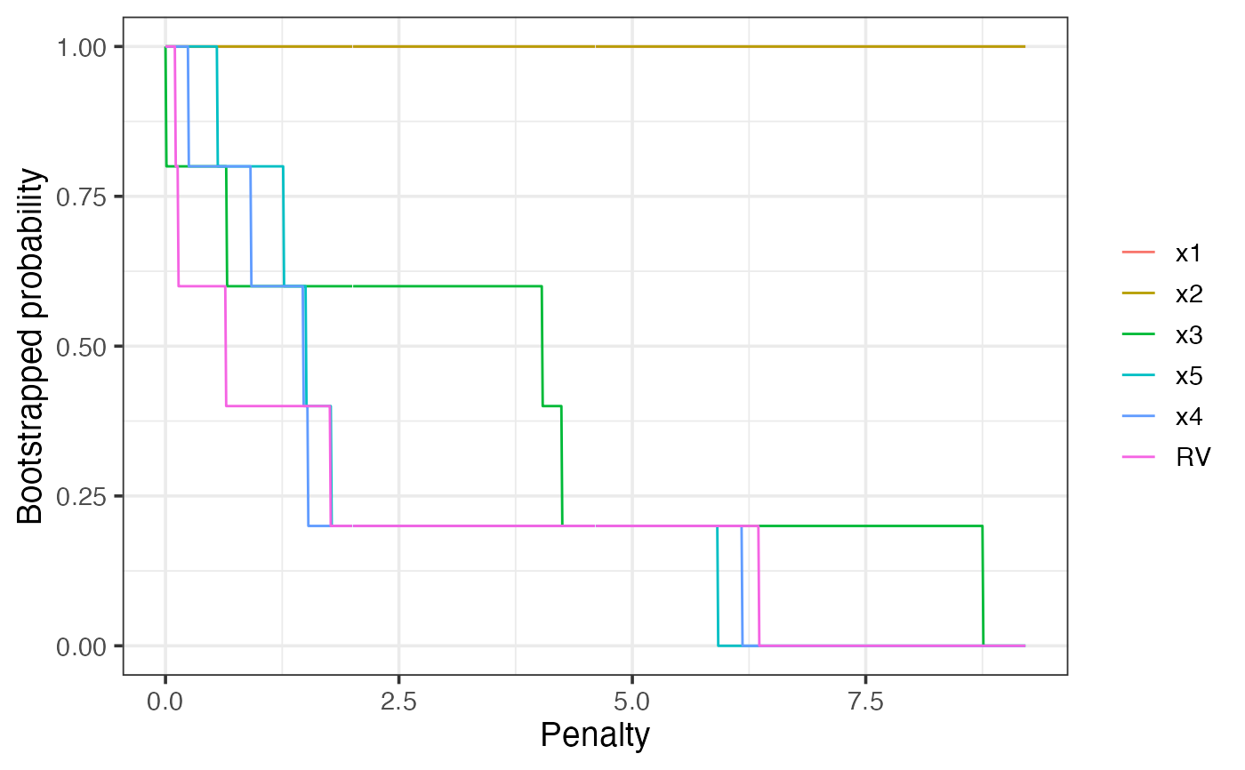
nbest	maximum number of models at each model size that will be considered for the lvk plot. Can also take a value of `"all"` which displays all models (default).
which	a vector specifying the plots to be output. Variable inclusion plots `which="vip"`; description loss against model size `which="lvk"`; bootstrapped description loss against model size `which="boot"`.
width	Width of the googleVis chart canvas area, in pixels. Default: 800.
height	Height of the googleVis chart canvas area, in pixels. Default: 400.
fontSize	font size used in googleVis chart. Default: 12.
left	space at left of chart (pixels?). Default: "50".
top	space at top of chart (pixels?). Default: "30".
chartWidth	googleVis chart area width. A simple number is a value in pixels; a string containing a number followed by `%` is a percentage. Default: `"60%"`
chartHeight	googleVis chart area height. A simple number is a value in pixels; a string containing a number followed by `%` is a percentage. Default: `"80%"`
axisTitlesPosition	Where to place the googleVis axis titles, compared to the chart area. Supported values: "in" - Draw the axis titles inside the the chart area. "out" - Draw the axis titles outside the chart area. "none" - Omit the axis titles.
dataOpacity	The transparency of googleVis data points, with 1.0 being completely opaque and 0.0 fully transparent.
options	a list to be passed to the googleVis function giving complete control over the output. Specifying a value for `options` overwrites all other plotting variables.
ylim	the y limits of the lvk and boot plots.
legend.position	the postion of the legend for classic plots. Default `legend.position="right"` alternatives include `legend.position="top"` and `legend.position="bottom"`
backgroundColor	The background colour for the main area of the chart. A simple HTML color string, for example: 'red' or '#00cc00'. Default: 'null' (there is an issue with GoogleCharts when setting 'transparent' related to the zoom window sticking - once that's sorted out, the default will change back to 'transparent')
text	logical, whether or not to add text labels to classic boot plot. Default = `FALSE`.
min.prob	when `text=TRUE`, a lower bound on the probability of selection before a text label is shown.
srt	when `text=TRUE`, the angle of rotation for the text labels. Default = 45.
max.circle	determines the maximum circle size. Default = 15.
print.full.model	logical, when `text=TRUE` this determines if the full model gets a label or not. Default=`FALSE`.
jitterk	amount of jittering of the model size in the lvk and boot plots. Default = 0.1.
seed	random seed for reproducible results
...	further arguments (currently unused)

Details

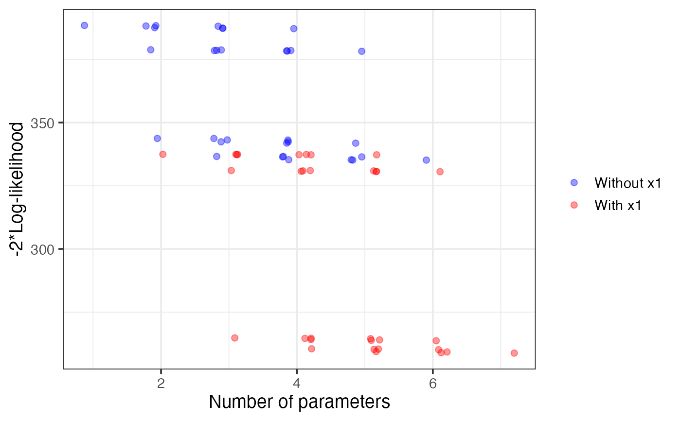
Specifying which = "lvk" generates a scatter plot where the points correspond to description loss is plot against model size for each model considered. The highlight argument is used to differentiate models that contain a particular variable from those that do not.

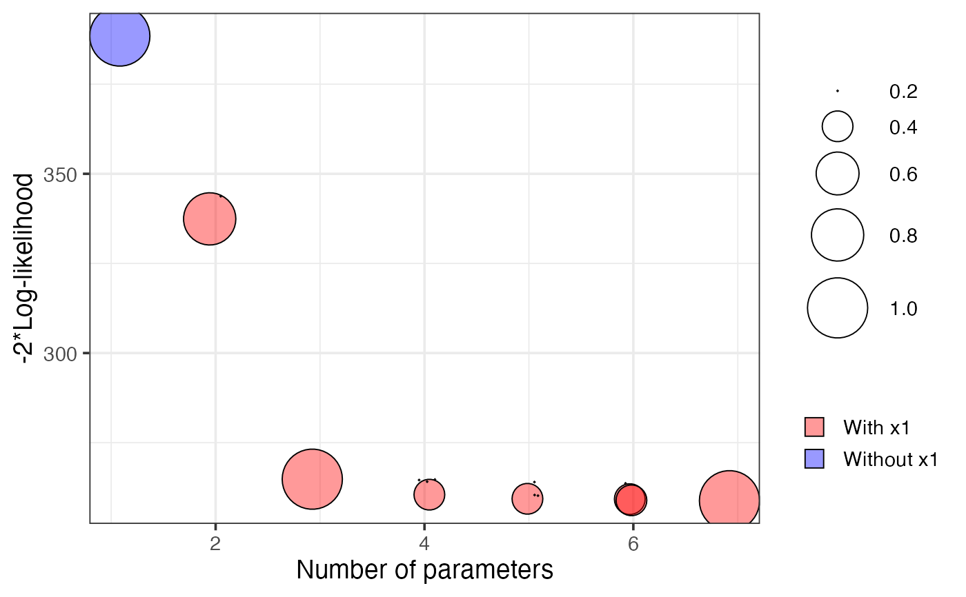
Specifying which = "boot" generates a scatter plot where each circle represents a model with a non-zero bootstrap probability, that is, each model that was selected as the best model of a particular dimension in at least one bootstrap replication. The area of each circle is proportional to the corresponding model's bootstrapped selection probability.

References

Mueller, S. and Welsh, A. H. (2010), On model selection curves. International Statistical Review, 78:240-256. doi: 10.1111/j.1751-5823.2010.00108.x

Murray, K., Heritier, S. and Mueller, S. (2013), Graphical tools for model selection in generalized linear models. Statistics in Medicine, 32:4438-4451. doi: 10.1002/sim.5855

Tarr G, Mueller S and Welsh AH (2018). mplot: An R Package for Graphical Model Stability and Variable Selection Procedures. Journal of Statistical Software, 83(9), pp. 1-28. doi: 10.18637/jss.v083.i09

Examples

n = 100
set.seed(11)
e = rnorm(n)
x1 = rnorm(n)
x2 = rnorm(n)
x3 = x1^2
x4 = x2^2
x5 = x1*x2
y = 1 + x1 + x2 + e
dat = data.frame(y,x1,x2,x3,x4,x5)
lm1 = lm(y~.,data=dat)
# \dontshow{
v1 = vis(lm1, B = 5, cores = 1, seed = 1)
plot(v1, highlight = "x1", which = "lvk")

plot(v1, which = "boot")

plot(v1, which = "vip")

# }
if (FALSE) {
v1 = vis(lm1, seed = 1)
plot(v1, highlight = "x1", which = "lvk")
plot(v1, which = "boot")
plot(v1, which = "vip")
}

Plot diagnostics for a vis object

Arguments

Details

References

See also

Examples