Overview of the simplified adaptive fence procedure.
The fence, first introduced by Jiang et al. (2008), is built around the inequality \[\hat{Q}(\alpha) - \hat{Q}(\alpha_{f}) \leq c,\] where \(\hat Q\) is an empirical measure of description loss, \(\alpha\) is a candidate model and \(\alpha_{f}\) is the baseline, full model. The procedure attempts to isolate a set of correct models that satisfy the inequality. A model \(\alpha^*\), is described as within the fence if \(\hat{Q}(\alpha^*) - \hat{Q}(\alpha_{f}) \leq c\). From the set of models within the fence, the one with minimum dimension is considered optimal. If there are multiple models within the fence at the minimum dimension, then the model with the smallest \(\hat{Q}(\alpha)\) is selected. For a recent review of the fence and related methods, see Jiang (2014).
The implementation we provide in the mplot package is inspired by the simplified adaptive fence proposed by Jiang et al. (2009), which represents a significant advance over the original fence method proposed by Jiang et al. (2008). The key difference is that the parameter \(c\) is not fixed at a certain value, but is instead adaptively chosen. Simulation results have shown that the adaptive method improves the finite sample performance of the fence.
The adaptive fence procedure entails bootstrapping over a range of values of the parameter \(c\). For each value of \(c\) a parametric bootstrap is performed under \(\alpha_f\). For each bootstrap sample we identify the smallest model inside the fence, \(\hat{\alpha}(c)\). Jiang et al. (2009) suggest that if there is more than one model, choose the one with the smallest \(\hat{Q}(\alpha)\). Define the empirical probability of selecting model \(\alpha\) for a given value of \(c\) as \(p^*(c,\alpha)=P^*\{\hat{\alpha}(c)=\alpha\}\). Hence, if \(B\) bootstrap replications are performed, \(p^*(c,\alpha)\) is the proportion of times that model \(\alpha\) is selected. Finally, define an overall selection probability, \(p^*(c)=\max_{\alpha\in\mathcal{A}}p^*(c,\alpha)\) and plot \(p^*(c)\) against \(c\) to find the first peak. The value of \(c\) at the first peak, \(c^*\), is then used with the standard fence procedure on the original data.
Our implementation is provided through the af() function
and associated plot methods. An example with the artificial data set is
generated using the following code.
The arguments indicate that we perform \(B = 150\) bootstrap resamples, over a grid of \(50\) values of the parameter \(c\). In this example, there is only one peak, and the choice of \(c^*=21.1\) is clear.
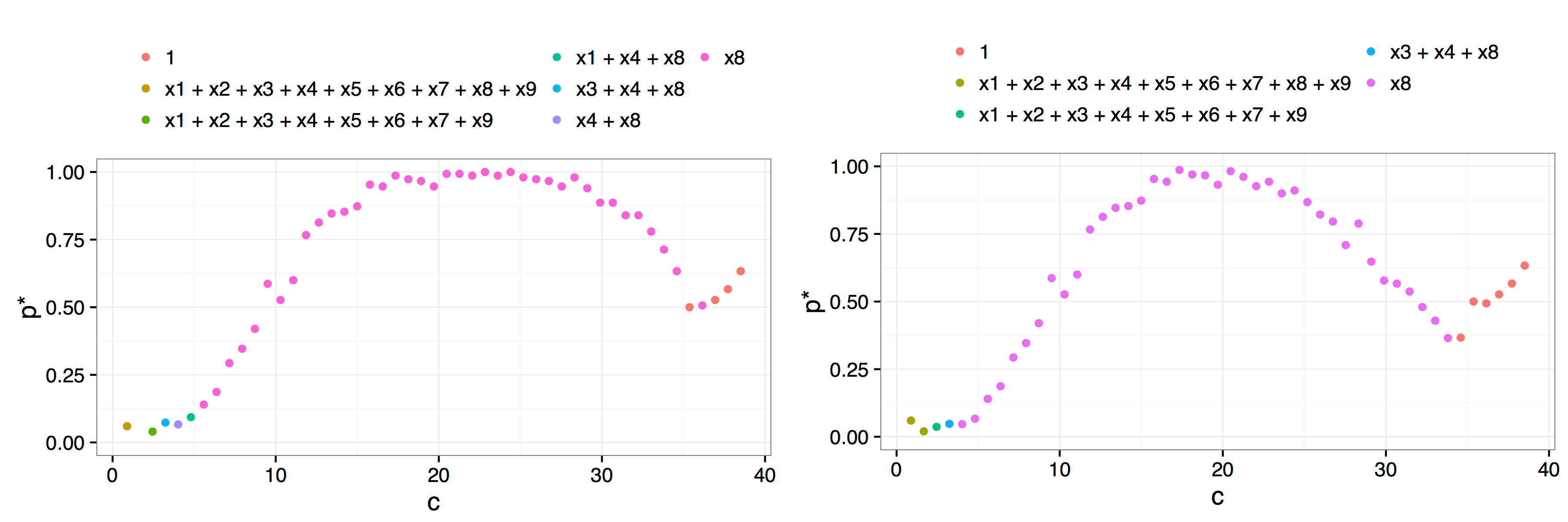
Result of a call to
plot(af.art, interactive = FALSE) with additional arguments
best.only = TRUE on the left and
best.only = FALSE on the right. The more rapid decay after
the \(x_8\) model is typical of using
best.only = FALSE where the troughs between
candidate/dominant models are more pronounced.
One might expect that there should be a peak corresponding to the full model at \(c=0\), but this is avoided by the inclusion of at least one redundant variable. Any model that includes the redundant variable is known to not be a true model and hence is not included in the calculation of \(p^*(c)\). This issue was first identified and addressed by Jiang et al. (2009).
There are a number of key differences between our implementation and the method proposed by Jiang et al. (2009). Perhaps the most fundamental difference is in the philosophy underlying our implementation. Our approach is more closely aligned with the concept of model stability than with trying to pick a single best model. This can be seen through the plot methods we provide. Instead of simply using the plots to identify the first peak, we add a legend that highlights which models were the most frequently selected for each parameter value, that is, for each \(c\) value we identify which model gave rise to the \(p^*(c)\) value. In this way, researchers can ascertain if there are regions of stability for various models. In the example given above, there is no need to even define a \(c^*\) value, it is obvious from the plot that there is only one viable candidate model, a regression of \(y\) on \(x_8\).
Our approach considers not just the best model of a given model size,
but also allows users to view a plot that takes into account the
possibility that more than one model of a given model size is within the
fence. The best.only = FALSE option when plotting the
results of the adaptive fence is a modification of the adaptive fence
procedure which considers all models of a particular size that are
within the fence when calculating the \(p^*(c)\) values. In particular, for each
value of \(c\) and for each bootstrap
replication, if a candidate model is found inside the fence, then we
look to see if there are any other models of the same size that are also
within the fence. If no other models of the same size are inside the
fence, then that model is allocated a weight of 1. If there are two
models inside the fence, then the best model is allocated a weight of
1/2. If three models are inside the fence, the best model gets a weight
of 1/3, and so on. After \(B\)
bootstrap replications, we aggregate the weights by summing over the
various models. The \(p^*(c)\) value is
the maximum aggregated weight divided by the number of bootstrap
replications. This correction penalises the probability associated with
the best model if there were other models of the same size inside the
fence. The rationale is that if a model has no redundant variables then
it will be the only model of that size inside the fence over a range of
values of \(c\). The result is more
pronounced peaks which can help to determine the location of the correct
peak and identify the optimal \(c^*\)
value or more clearly differentiate regions of model stability. This can
be seen in the right hand panel of the figure above.
Another key difference is that our implementation is designed for linear and generalised linear models, rather than mixed models. As far as we are aware, this is the first time fence methods have been applied to such models. There is potential to add mixed model capabilities to future versions of the mplot package, but computational speed is a major hurdle that needs to be overcome. The current implementation is made computationally feasible through the use of the leaps and bestglm packages and the use of parallel processing (Lumley & Miller, 2009; McLeod & Xu, 2014).
We have also provided an optional initial stepwise screening method
that can help limit the range of \(c\)
values over which to perform the adaptive fence procedure. The initial
stepwise procedure performs forward and backward stepwise model
selection using both the AIC and BIC. From the four candidate models, we
extract the size of smallest and largest models, \(k_L\) and \(k_U\) respectively. To obtain a sensible
range of \(c\) values we consider the
set of models with dimension between \(k_L-2\) and \(k_U+2\). Due to the inherent limitations of
stepwise procedures, it can be useful to check
initial.stepwise = FALSE with a small number of bootstrap
replications over a sparse grid of \(c\) values to ensure that the
initial.stepwise = TRUE has produced a reasonable
region.