Lecture 3

class: center, middle, inverse, title-slide

# Lecture 3
## Regularisation procedures with glmnet
### Samuel Müller and Garth Tarr

---

## Review Lecture 2

1. More on .blue[stepwise procedures]
    - Forward stepwise
    - Issues with stepwise procedures
2. .red[Exhaustive search for linear models]
    - The `leaps` package
3. .red[Exhaustive search for generalised linear models]
    - Logistic regression
    - Marginality principle
    - The `bestglm` package

---

## Overview

1. Regularisation with glmnet
2. .blue[Lasso regression]
3. .red[Ridge regression]
4. Comparing ridge and lasso
5. .blue[Elastic-net]
6. Cross-validation for model selection
7. Selecting `$\lambda$`
8. .blue[Adaptive lasso]

---
class: segue

# Regularisation with glmnet

---

## Regularisation methods with `glmnet`

.blockquote[
Regularisation methods **shrink** estimated regression coefficients by imposing a penalty on their sizes
]

- There are different choices for the .blue[.bold[penalty]]
- The penalty choice drives the properties of the method

In particular, `glmnet` implements

- .blue[.bold[Lasso regression]] using a `$L_1$` penalty
- .red[.bold[Ridge regression]] using a `$L_2$` penalty
- .orange[.bold[Elastic-net]] using both, an `$L_1$` and an `$L_2$` penalty
- **Adaptive lasso**, it takes advantage of feature weights

---
class: segue

# Lasso regression

---

## Least squares with `$L_1$` penalty

If the response vector `$\boldsymbol{y} \in \Bbb{R}^n$` and design matrix `$\boldsymbol{X}\in\text{mat}(n,p)$` have (columnwise) zero mean (and therefore no intercept is fitted)
`$$\hat{\boldsymbol{\beta}}_{\text{lasso}} = \hat{\boldsymbol{\beta}}_{\text{lasso}}({\color{red}\lambda}) = \operatorname{argmin}_{\boldsymbol{\beta} \in \Bbb{R}^p} \{ (\boldsymbol{y}-\boldsymbol{X}\boldsymbol{\beta})^T (\boldsymbol{y}-\boldsymbol{X}\boldsymbol{\beta}) + {\color{red}\lambda} \, \color{blue}{||\boldsymbol{\beta}||_1}\},$$`
where the positive tuning parameter `$\lambda$` controls the shrinkage.

This optimisation problem is equivalent to solving
`$$\text{minimise } \operatorname{RSS}(\boldsymbol{\beta}) = (\boldsymbol{y}-\boldsymbol{X}\boldsymbol{\beta})^T (\boldsymbol{y}-\boldsymbol{X}\boldsymbol{\beta}) \text{ subject to } {\color{blue}{\sum_{j=1}^p |\beta_j|}} \leq t.$$`
There exists a one-to-one map between `$\lambda$` and `$t$` through `$$t = \sum_{j=1}^p |\hat\beta_{\text{lasso},j}(\lambda)|.$$`
Clearly, the smaller `$t$` and the larger `$\lambda$`, respectively, the more `$\hat{\boldsymbol{\beta}}_{\text{lasso}}$` will be shrunk towards zero.

---
class: eg

## Example: Diabetes

- We consider the `diabetes` data and we only analyse main effects
- The data from the `lars` package is the same as the `mplot` package but is structured and scaled differently

```r
data("diabetes", package = "lars")
names(diabetes)  # list, slot x has 10 main effects
```

```
## [1] "x"  "y"  "x2"
```

```r
dim(diabetes)
```

```
## [1] 442   3
```

```r
x = diabetes$x
y = diabetes$y
```

---
class: eg

## Example: Diabetes

```r
class(x) = NULL # remove the AsIs class; otherwise single boxplot drawn
boxplot(x, cex.axis = 2)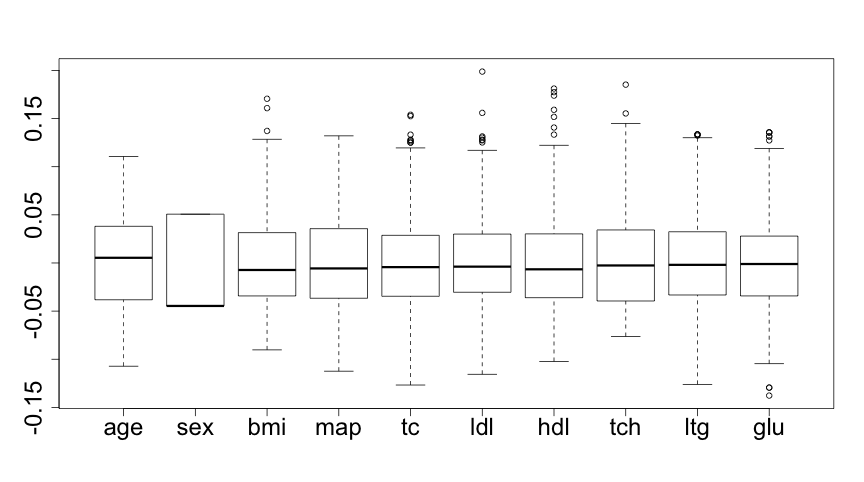
```

![](lec03_files/figure-html/unnamed-chunk-1-1.png)

---
class: eg code90

## Example: Diabetes

.scroll-output[

```r
lm.fit = lm(y ~ x)  #least squares fit for the full model first
summary(lm.fit)
```

```
## 
## Call:
## lm(formula = y ~ x)
## 
## Residuals:
## Min 1Q Median 3Q Max 
## -155.829 -38.534 -0.227 37.806 151.355 
## 
## Coefficients:
## Estimate Std. Error t value Pr(>|t|) 
## (Intercept) 152.133 2.576 59.061 < 2e-16 ***
## xage -10.012 59.749 -0.168 0.867000 
## xsex -239.819 61.222 -3.917 0.000104 ***
## xbmi 519.840 66.534 7.813 4.30e-14 ***
## xmap 324.390 65.422 4.958 1.02e-06 ***
## xtc -792.184 416.684 -1.901 0.057947 . 
## xldl 476.746 339.035 1.406 0.160389 
## xhdl 101.045 212.533 0.475 0.634721 
## xtch 177.064 161.476 1.097 0.273456 
## xltg 751.279 171.902 4.370 1.56e-05 ***
## xglu 67.625 65.984 1.025 0.305998 
## ---
## Signif. codes: 0 '***' 0.001 '**' 0.01 '*' 0.05 '.' 0.1 ' ' 1
## 
## Residual standard error: 54.15 on 431 degrees of freedom
## Multiple R-squared: 0.5177,	Adjusted R-squared: 0.5066 
## F-statistic: 46.27 on 10 and 431 DF, p-value: < 2.2e-16
```
]

---

## Fitting a lasso regression
Lasso regression with the `glmnet()` function in `library(glmnet)` has as a first argument the design matrix and as a second argument the response vector, i.e.

```r
library(glmnet)
lasso.fit = glmnet(x,y)
```

---

### Comments
- `glmnet.fit` is an object of class glmnet that contains all the relevant information of the fitted model for further use 
- Various methods are provided for the object such as `coef`, `plot`, `predict` and `print` that extract and present useful object information
- We will later see that cross-validation can be used to choose a good value for `$\lambda$` through using the function `cv.glmnet`

```r
set.seed(1) # to get a reproducable lambda.min value
lasso.cv = cv.glmnet(x, y)
lasso.cv$lambda.min
```

```
## [1] 0.9958377
```

---
class: eg

## Lasso regression coefficients
Clearly the regression coefficients are smaller for the .blue[lasso regression] (this slide) than for .red[least squares] (next slide)

```r
round(coef(lasso.fit,s=c(5,1,0.5,0)),2)
```

```
## 11 x 4 sparse Matrix of class "dgCMatrix"
##                   1       2       3       4
## (Intercept)  152.13  152.13  152.13  152.13
## age            .       .       .      -9.22
## sex          -45.33 -195.90 -216.37 -239.06
## bmi          509.05  522.05  525.08  520.46
## map          217.20  296.19  308.30  323.62
## tc             .    -101.86 -160.96 -716.48
## ldl            .       .       .     418.45
## hdl         -147.74 -223.22 -180.46   65.39
## tch            .       .      66.10  164.56
## ltg          446.35  513.57  524.22  723.74
## glu            .      53.86   61.15   67.54
```

---

## Lasso regression vs least squares

```r
round(coef(lm.fit),2)
```

```
## (Intercept)        xage        xsex        xbmi        xmap 
##      152.13      -10.01     -239.82      519.84      324.39 
##         xtc        xldl        xhdl        xtch        xltg 
##     -792.18      476.75      101.04      177.06      751.28 
##        xglu 
##       67.63
```

```r
beta.lasso = coef(lasso.fit,s=1)
sum(abs(beta.lasso[-1]))
```

```
## [1] 1906.658
```

```r
beta.ls = coef(lm.fit)
sum(abs(beta.ls[-1]))
```

```
## [1] 3460.005
```

---
class: eg

## Lasso coefficient plot

```r
plot(lasso.fit, label = TRUE, cex.axis = 1.5, cex.lab = 1.5)
```

![](lec03_files/figure-html/unnamed-chunk-6-1.png)

---

## We observe that the lasso

- Can shrink coefficients exactly to zero
- Simultaneously estimates and selects coefficients
- Paths are not necessarily monotone (e.g. coefficients for `hdl` in above table for different values of `s`)

---

## Further remarks on lasso

- .blue[.bold[lasso]] is an acronym for **l**east **a**bsolute **s**election and **s**hrinkage **o**perator
- Theoretically, when the tuning parameter `$\lambda=0$`, there is no bias and `$\hat{\boldsymbol{\beta}}_{\text{lasso}} = \hat{\boldsymbol{\beta}}_{\text{LS}}$` ( `$p\leq n$` ) however, `glmnet` *approximates* the solution
- When `$\lambda=\infty$`, we get `$\hat{\boldsymbol{\beta}}_{\text{lasso}} = 0$` `$\Rightarrow$` an estimator with zero variance
- For `$\lambda$` in between, we are balancing bias and variance 
- As `$\lambda$` increases, more coefficients are set to zero (less variables are selected), and among the nonzero coefficients, more shrinkage is employed

---

## Lasso without penalizing the intercept

- The intercept is often treated differently to slopes
- `glmnet` (by default) .blue[does not penalise the intercept] and solves
`$$\text{minimise }\operatorname{RSS}(\color{blue}{\beta_0},\color{red}{\beta_1,\ldots,\beta_p}) + \lambda\,\sum_{\color{red}{j=1}}^{\color{red}{p}} |\beta_j|$$`
- Typically columns of `$\boldsymbol{X}$` are scaled to have sample variance 1 (or `$\sum_{i=1}^n x_{ij}^2 = n$`), to make sure that all regressors contribute equally to the penalty term `$\sum_{j=1}^p|\beta_j|$`
- Default option: `glmnet(..., standardize=TRUE, ...)`
- The penalty term `$||\beta||_{1}=\sum_{j=1}^p|\beta_j|$` is not fair if the predictor variables are not on the same scale
- On the other hand, deliberately changing the scale, can have great advantages as we will see later

---

## Why does the lasso give zero coefficients?

.footnote[
This figure is taken from James, Witten, Hastie, and Tibshirani (2013) "An Introduction to Statistical Learning, with applications in R" with permission from the authors.
]

---
class: segue

# Ridge regression

---

## Ridge is least squares with `$L_2$` penalty

- As the lasso, .red[ridge regression] shrinks the estimated regression
coefficients by imposing a penalty on their sizes
`$$\text{minimise } \operatorname{RSS}(\boldsymbol{\beta}) = (\boldsymbol{y}-\boldsymbol{X}\boldsymbol{\beta})^T (\boldsymbol{y}-\boldsymbol{X}\boldsymbol{\beta}) \text{ subject to } {\color{red}{\sum_{j=1}^p \beta_j^2}} \leq t,$$`
where the positive tuning parameter `$\lambda$` controls the shrinkage
- However, unlike the lasso, .red[ridge regression does not shrink the parameters all the way to zero]
- Ridge coefficients have closed form solution (even when `$n < p$`)
$$
\hat{\boldsymbol{\beta}}_{\text{ridge}}(\lambda) = (\boldsymbol{X}^T\boldsymbol{X}+\lambda\boldsymbol{I})^{-1}\boldsymbol{X}^T\boldsymbol{y}
$$

---

## Fitting a ridge regression

Ridge regression with the `glmnet()` function by changing one of its default options to `alpha=0`

```r
ridge.fit = glmnet(x, y, alpha = 0)
ridge.cv = cv.glmnet(x, y, alpha = 0)
ridge.cv$lambda.min
```

```
## [1] 4.956308
```

### Comments
- In general, the optimal `$\lambda$` for ridge is very different than the optimal `$\lambda$` for the lasso
- The scale of `$\sum\beta_j^2$` and `$\sum|\beta_j|$` is very different
- `$\color{orange}{\alpha}$` is known as the elastic-net mixing parameter

---
class: segue

# Comparing ridge and lasso

---

## Three types of regression coefficients

- Simulation with `$n=50$` and `$p=30$`, `$\boldsymbol{X}$` with iid components from `$N(0,1)$`
- Choose 10 coefficients .blue[zero], 10 coefficients .red[small between 0.2 and 0.4] and 10 coefficients are  .orange[large between 0.6 and 1]

```r
set.seed(2014); n = 50; p = 30
X = matrix(rnorm(n*p), nrow = n)
beta = c(rep(0, 10), runif(10, 0.2, 0.4), runif(10, 0.6, 1))
plot(table(round(beta,2)), xlab="True coefficients", ylab = "Count")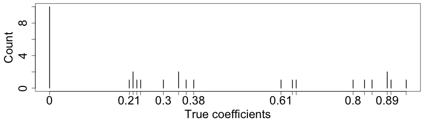
```

![](lec03_files/figure-html/unnamed-chunk-8-1.png)

---

## Comparing estimates

Here, ridge with `$\lambda = 0.6$` and Lasso with `$\lambda = 0.1$`: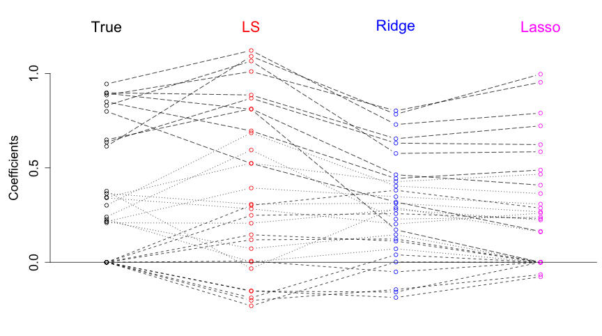

![](lec03_files/figure-html/unnamed-chunk-9-1.png)

---

## Bias, Variance and MSE for ridge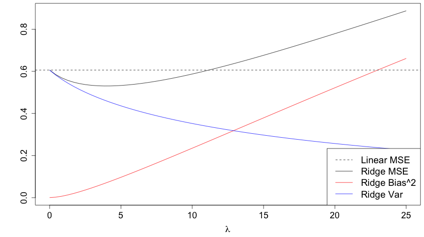

![](lec03_files/figure-html/unnamed-chunk-10-1.png)

---

## Bias, Variance and MSE for lasso

![](lec03_files/figure-html/unnamed-chunk-11-1.png)

---

## Simulation study: Remarks

- The range of `$\lambda$` values where the lasso does better than LS is completely different to the range of `$\lambda$` values where ridge regression does better than LS
- To compare different types of estimators, the concept of .blue[degree of freedom] should be used and not the tuning parameter

---

## Degrees of freedom

- There are many definitions of what the .blue[degrees of freedom] (df) are 
- Here, measure the .blue[effective number of parameters] of an estimate
- Formally, for an iid regression model, the df of an estimate `$\hat{\boldsymbol{y}}$` is 
$$
\text{df}(\hat{\boldsymbol{y}}) = \frac{1}{\sigma^2}\sum_{i=1}^n\text{Cov}(\hat y_i,y_i) 
$$
- The higher the correlation between the `$i$`th fitted value and the `$i$`th data point, the more adaptive the estimate, and so the higher its degrees of freedom

### Results (without proof)

- For LS regression, `$\text{df}(\hat{\boldsymbol{y}}) = p$`
- For ridge regression, `$\text{df}(\hat{\boldsymbol{y}}) = \text{trace}(\boldsymbol{X}(\boldsymbol{X}^T\boldsymbol{X}+\lambda\boldsymbol{I})^{-1}\boldsymbol{X}^T)$`
- For lasso regression, `$\text{df}(\hat{\boldsymbol{y}}) = \text{E}\left[\sum_{j=1}^p \text{sign}(|\hat\beta_{\text{lasso},j}|)\right]$`

---
class: segue

# Elastic-net

---

## Elastic-net: best of both worlds?

- Minimising the (penalised) log-loglikelihood in linear regression with iid errors is equivalent to minimising the (penalised) RSS
- More generally, the elastic-net minimises the following objective function over `$\color{blue}{\beta_0}$` and `$\color{red}{\boldsymbol{\beta}}$` over a grid of values of `$\lambda$` covering the entire range
`$$\frac{1}{n} \sum_{i=1}^{N} w_i l(y_i,\color{blue}{\beta_0}+\color{red}{\boldsymbol{\beta}}^T \boldsymbol{x}_i) + \lambda\left[(1-\color{orange}{\alpha}) \color{red}{\sum_{j=1}^p\beta_j^2 } + \color{orange}{\alpha} \color{red}{\sum_{j=1}^p|\beta_j| } \right]$$`
- This is general enough to include logistic regression, generalised linear models and Cox regression, where `$l(y_i)$` is the log-likelihood of observation `$i$` and `$w_i$` an optional observation weight

---

### Comments
- The .red[ridge] penalty tends to shrink the coefficients of correlated predictors towards each other
- While the .blue[lasso] tends to pick one of them and discard the others 
- The `glmnet` algorithms use cyclical coordinate descent and a range of tricks to compute the solution path very quickly

---

## Some additional `glmnet` options

`x` input matrix, of dimension `nobs x nvars` `$=n\times p$`

`y` response variable. Quantitative for `family = "gaussian"`. For `family = "binomial"` simplest when a factor with two levels. See `help(glmnet)` for more options and types of models

`family="gaussian"` or `"binomial"`, `"poisson"`, `"multinomial"`, `"cox"`, `"mgaussian"`

`weights` an optional vector of observation weights, the `$w_i$`'s above

`nlambda = 100` The number of `$\lambda$` values - default is 100

`lambda.min.ratio` Smallest value for `$\lambda$`, as a fraction of `lambda.max`, the (data derived) entry value (i.e. the smallest `$\lambda$` value for which all coefficients are zero). WARNING: a very small value of `lambda.min.ratio` can lead to a saturated fit, which is undefined for `"binomial"` and `"multinomial"` models

---

## Some additional `glmnet` options

`lambda` A user supplied lambda sequence. WARNING: use with care. Do not supply
a single value for lambda (for predictions after CV use `predict()` instead)

`standardize = TRUE` Logical flag for x variable standardisation, prior to fitting the model sequence. The coefficients are always returned on the original scale

`intercept = TRUE` By default an intercept is fitted

`penalty.factor` Separate penalty factors can be applied to each of the `$j=1,\ldots,p$` coefficients. This is a number that multiplies lambda to allow differential shrinkage. If 0 for some variables, there is no shrinkage, and if infinity then these variables will be excluded

---
class: eg

## Logistic regression example
The `glmnet` package has a range of simulated data sets. `BinomialExample` consists of a design matrix `x` and response vector `y`, accessible after running `data(BinomialExample)`:

```r
rm(x)
rm(y) # clear previous x and y vars
data("BinomialExample", package = "glmnet")
dim(x)
```

```
## [1] 100  30
```

```r
table(y)
```

```
## y
##  0  1 
## 44 56
```

---
class: eg

## Logistic regression example

```r
enet.fit = glmnet(x, y, family = "binomial", alpha=0.5)
plot(enet.fit, xvar = "dev", label = TRUE)
```

![](lec03_files/figure-html/unnamed-chunk-13-1.png)

---

## How to assess logistic regresion models?

For logistic regression, `cv.glmnet` has similar arguments and usage as when working with Gaussian errors

There are some differences in `type.measure` but we just focus on those model assessment measures most relevant for logistic regression:

- `deviance` is the actual deviance
- `mae` is the mean absolute error
- `class` gives the model misclassification error
- `auc` (for two-class logistic regression ONLY) gives the area under the ROC curve

---
class: eg

## Minimising the misclassification error

```r
enet.cv = cv.glmnet(x, y, family = "binomial", alpha = 0.5, 
                    type.measure = "class")
c(enet.cv$lambda.min,enet.cv$lambda.1se)
```

```
## [1] 0.02450038 0.03901154
```

```r
plot(enet.cv)
```

![](lec03_files/figure-html/unnamed-chunk-14-1.png)

---

## Some R packages for regularized (generalized) linear mixed models (G)LMM

- `lmmlasso` fits (gaussian) LMMs for high-dimensional data (n<<p) using a Lasso-type approach for the fixed-effects parameter; we refer to Müller, Scealy, and Welsh (2013) for a review on mixed model selection
- `glmmLasso` does variable selection for GLMs by L1-penalized estimation
- `rpql` does joint selection in GLMMs using penalized likelihood methods as described in Hui, Müller, and Welsh (2017)

---
class: segue

# Cross-validation for model selection

---

## Resampling procedures

- .orange[Cross-validation (CV)] and bootstrapping are the two most popular classes of .blue[resampling methods] in model building
- In model building, resampling is often used to
 - assess the stability of a model
 - infer on model parameters (tests, confidence intervals, point estimates, bias)
- measure .blue[prediction error]

---

## Cross-validation algorithms

- .orange[Cross-validation] schemes can be implemented in most statistical frameworks and for most estimation procedures
- The key principle of CV is to .blue[split the data] into a .blue[training set] and a .red[validation set] 
- .blue[Estimators] are .blue[built on the training set]
- .red[Validation set] is used .red[to] validate/.red[assess] the .red[performance] of the estimators, e.g. estimating their prediction risk 
- This training / validation splitting is repeated several times

---

## Cross-validation algorithms

The most popular .orange[cross-validation schemes] are,

- .blue[Hold-out CV] which is based on a single split of the data for training and validation
- `$\color{red}{k}$`-fold CV: the data is split into `$k$` subsamples. Each subsample is successively removed for validation, the remaining data being used for training
- .blue[Leave-one-out] (LOOCV) which corresponds to `$n$`-fold CV
- Leave- `$q$`-out (also called delete- `$q$`-CV), where every possible subset of cardinality
`$q$` of the data is removed for validation, the remaining data being used for training

---

## Estimating expected prediction error with `$k$`-fold CV

- Recall, in `$k$`-fold CV the data is split into `$k$` subsamples (the `$k$` folds)
- Each subsample is successively removed for .red[validation], the remaining data being used for .blue[training]
- Thus, for each of the `$k$` folds `$f=1,\ldots,k$`,  `$\iota_f\subset\{1,\ldots,n\}$` denotes the `$n_f = |\iota_f|$` observations in the `$f$`th fold and we calculate
`$$\text{CV}_{(k)} = \frac{1}{k} \sum_{f=1}^k \text{MSE}_f = \frac{1}{k}\sum_{f=1}^k \frac{1}{n_f}\sum_{i\in \iota_f} [y_i - \hat y_{\alpha i}(-\iota_f)]^2$$`
- Similarly, for estimating classification errors

---

## Choice of `$k$` affects the quality of the CV error

- If `$\color{blue}{k=2}$`: split-sample CV - CV error estimates .blue[biased] upwards because only half the data used in the training samples
- If `$\color{red}{k=n}$`: LOOCV - CV estimates have .red[high variance] because in the above equation a total of `$n$` positively correlated quantities are averaged;
- .blue[Standard choices] are `$\color{blue}{k=10}$` (default in `cv.glmnet` through option `nfolds=10`) or `$k=5$`: 
    - This balances bias and variance 
    - It is generally believed that these choices give good estimates of prediction error 
    - However, there is not really any theory supporting this
- The `$k$` partly overlapping training sets can be used to learn more about the stability of selected models, simply by selecting one or more models for each of the `$f$` training sets

---
class: segue

# Selecting `$\lambda$`

---

## How to best choose `$\lambda$`?

- Many options!
- .blue[Use information criteria along the lasso], ridge, or elastic-net .blue[path]
- Use cross-validation
    - as an alternative to `lambda.min` often `lambda.1se` does give better performance in terms of prediction
    - `lambda.1se` is the largest `$\lambda$` at which the MSE is within one standard error of the minimal MSE (at `lambda.min`)

---
class: eg

### Diabetes example

```r
x = as.matrix(diabetes)[, -11]
y = as.matrix(diabetes)[, 11]
lasso.fit = glmnet(x, y)
length(lasso.fit$lambda)
```

```
## [1] 100
```

```r
lasso.predict = predict(lasso.fit, newx = x)
dim(lasso.predict)
```

```
## [1] 442 100
```

---
class: eg

### Diabetes example

```r
lasso.bic = rep(0, 100)
sigma.hat = summary(lm(y ~ x))$s
for (m in 1:100) {
    yhat = lasso.predict[, m]
    k = lasso.fit$df[m]
    lasso.bic[m] = sum((y - yhat)^2)/(sigma.hat^2) + log(422) * k
}
which.min(lasso.bic)
```

```
## [1] 26
```

```r
lasso.fit$lambda[26]
```

```
## [1] 4.41218
```

---
class: segue

# Adaptive lasso

---

## The weighted lasso

- Several extensions since its initial presentation by Tibshirani (1996) 
- A particular variant is the weighted lasso for `$p > n$`, which has the adaptive lasso (Zou, 2006) for `$p < n$` as a special case 
- Weighted lasso generalises the lasso through (data dependent) weights
- In `glmnet` simply specify `penalty.factor = ` `$\boldsymbol{w}$`, with components `$\hat{w}_j$` given below
- The adaptive lasso minimises the objective function
`$${\|\boldsymbol{y} -\boldsymbol{X}\boldsymbol{\beta} \|^2 + \lambda \sum_{j=1}^p \hat{w}_j}|\beta_j|,\quad \hat{w}_j = 1/|\hat{\beta}_{\text{LS},j}|$$`
- Here, `$\hat{\beta}_{\text{LS},j}$`, `$j=1,\ldots,p$`, denotes the ordinary least squares estimate after regressing `$\boldsymbol{y}$` on `$\boldsymbol{X}$`

---

## Writing the weighted lasso as the lasso

- The weighted  lasso turns the variable selection problem into optimally selecting the tuning parameter `$\lambda$`
- Weighted lasso equation (above) is minimised by using the standard lasso procedure: 
    - First,  we transform the covariates, i.e., `$x_{ij} \mapsto x_{ij}/\hat{w}_j = x^*_{ij}$`, `$z_{ij} \mapsto z_{ij}/\hat{w}_j = z^*_{ij}$`, and define `$\gamma_j = \hat{w}_j\beta_j$` 
    - Define `$\boldsymbol{X}^* = (\boldsymbol{x}_{1}^*,\ldots,\boldsymbol{x}_{p}^*)$`. Then we solve for `$\hat{\boldsymbol{\gamma}}$` by minimising
$$
||\boldsymbol{y} -\boldsymbol{X}^*\boldsymbol{\gamma} ||^2 + \lambda \sum_{j=1}^p |\gamma_j|, 
$$
and obtain the final estimates through the transformation `$\hat{\beta}_j = \hat{\gamma}_j / \hat{w}_j$`

---

## The magic is in the weights

- Although the adaptive lasso uses weights `$\hat{w}_j = 1/|\hat{\beta}_{\text{LS},j}|$`, any appropriate data dependent weights can be used
- Larger weights make it more likely that variables are excluded early in the lasso path   
- Using different weights to `$|\hat{\beta}_{\text{LS},j}|^{-1}$` has been explored recently:
    - estimating parameters from ridge regression (when `$p > n$`)
    - choosing weights that incorporate prior knowledge or relevant external information on the covariates, Charbonnier, Chiquet, and Ambroise (2010), Bergersen, Glad, and Lyng (2011)
    - using weights that are proportional to measures of significance such as p-values, q-values, partial correlation coefficients etc as in  Garcia and Müller (2014)
    - using weights from stability measures such as exclusion frequencies from repeatedly subsetting the columns of the design matrix as in  Garcia and Müller (2016)

---
class: font100 columns-2

## References

<a name=bib-Bergersen2011></a>[Bergersen, L. C, I. K.
Glad and H. Lyng](#cite-Bergersen2011) (2011). "Weighted
lasso with data integration". In: _Statistical
Applications in Genetics and Molecular Biology_ 10.1, pp.
1544-6115. DOI:
[10.2202/1544-6115.1703](https://doi.org/10.2202%2F1544-6115.1703).

<a name=bib-Charbonnier2010></a>[Charbonnier, C, J.
Chiquet and C. Ambroise](#cite-Charbonnier2010) (2010).
"Weighted-Lasso for structured network inference from
time course data". In: _Statistical Applications in
Genetics and Molecular Biology_ 9.1, pp. 1544-6115. DOI:
[10.2202/1544-6115.1519](https://doi.org/10.2202%2F1544-6115.1519).

<a name=bib-Garcia2014></a>[Garcia, T. P. and S.
Müller](#cite-Garcia2014) (2014). "Influence of measures
of significance based weights in the weighted lasso". In:
_Journal of the Indian Society of Agricultural
Statistics_ 68.2, pp. 131-144.

<a name=bib-Garcia2016></a>[Garcia, T. P. and S.
Müller](#cite-Garcia2016) (2016). "Cox regression with
exclusion frequency-based weights to identify
neuroimaging markers relevant to Huntington's disease
onset". In: _Annals of Applied Statistics_ 10.4, pp.
2130-2156.

<a name=bib-Hui2017></a>[Hui, F. K. C, S. Müller and A.
H. Welsh](#cite-Hui2017) (2017). "Joint Selection in
Mixed Models using Regularized PQL". In: _Journal of the
American Statistical Association_, p. 34 pages. DOI:
[10.1080/01621459.2016.1215989](https://doi.org/10.1080%2F01621459.2016.1215989).

<a name=bib-James2013></a>[James, G, D. Witten, T.
Hastie, et al.](#cite-James2013) (2013). _An introduction
to statistical learning with applications in R_. New
York, NY: Springer. ISBN: 9781461471370. URL:
[http://www-bcf.usc.edu/~gareth/ISL/](http://www-bcf.usc.edu/~gareth/ISL/).

<a name=bib-Mueller2013></a>[Müller, S, J. L. Scealy and
A. H. Welsh](#cite-Mueller2013) (2013). "Model Selection
in Linear Mixed Models". In: _Statistical Science_ 28.2,
pp. 135-167. DOI:
[10.1214/12-STS410](https://doi.org/10.1214%2F12-STS410).

<a name=bib-Tibshirani1996></a>[Tibshirani,
R.](#cite-Tibshirani1996) (1996). "Regression shrinkage
and selection via the lasso". In: _Journal of the Royal
Statistical Society: Series B (Methodological)_, pp.
267-288. URL:
[http://www.jstor.org/stable/10.2307/2346178](http://www.jstor.org/stable/10.2307/2346178).

<a name=bib-Zou2006></a>[Zou, H.](#cite-Zou2006) (2006).
"The adaptive lasso and its oracle properties". In:
_Journal of the American Statistical Association_
101.476, pp. 1418-1429. DOI:
[10.1198/016214506000000735](https://doi.org/10.1198%2F016214506000000735).

---
class: code60 columns-2

```r
devtools::session_info(include_base = FALSE)
```

```
## Session info --------------------------------------------------------------------------------------
```

```
##  setting  value                       
##  version  R version 3.5.0 (2018-04-23)
##  system   x86_64, darwin15.6.0        
##  ui       X11                         
##  language (EN)                        
##  collate  en_AU.UTF-8                 
##  tz       Australia/Sydney            
##  date     2018-06-10
```

```
## Packages ------------------------------------------------------------------------------------------
```

```
##  package        * version date       source                              
##  assertthat       0.2.0   2017-04-11 CRAN (R 3.5.0)                      
##  backports        1.1.2   2017-12-13 CRAN (R 3.5.0)                      
##  base           * 3.5.0   2018-04-24 local                               
##  bibtex           0.4.2   2017-06-30 CRAN (R 3.5.0)                      
##  bindr            0.1.1   2018-03-13 CRAN (R 3.5.0)                      
##  bindrcpp         0.2.2   2018-03-29 CRAN (R 3.5.0)                      
##  codetools        0.2-15  2016-10-05 CRAN (R 3.5.0)                      
##  compiler         3.5.0   2018-04-24 local                               
##  datasets       * 3.5.0   2018-04-24 local                               
##  devtools         1.13.5  2018-02-18 CRAN (R 3.5.0)                      
##  digest           0.6.15  2018-01-28 CRAN (R 3.5.0)                      
##  doRNG            1.6.6   2017-04-10 CRAN (R 3.5.0)                      
##  dplyr            0.7.5   2018-05-19 CRAN (R 3.5.0)                      
##  evaluate         0.10.1  2017-06-24 CRAN (R 3.5.0)                      
##  foreach        * 1.4.4   2017-12-12 CRAN (R 3.5.0)                      
##  formatR          1.5     2017-04-25 CRAN (R 3.5.0)                      
##  glmnet         * 2.0-16  2018-04-02 CRAN (R 3.5.0)                      
##  glue             1.2.0   2017-10-29 CRAN (R 3.5.0)                      
##  graphics       * 3.5.0   2018-04-24 local                               
##  grDevices      * 3.5.0   2018-04-24 local                               
##  grid             3.5.0   2018-04-24 local                               
##  htmltools        0.3.6   2017-04-28 CRAN (R 3.5.0)                      
##  httpuv           1.4.3   2018-05-10 cran (@1.4.3)                       
##  httr             1.3.1   2017-08-20 CRAN (R 3.5.0)                      
##  iterators        1.0.9   2017-12-12 CRAN (R 3.5.0)                      
##  jsonlite         1.5     2017-06-01 CRAN (R 3.5.0)                      
##  knitcitations  * 1.0.8   2017-07-04 CRAN (R 3.5.0)                      
##  knitr            1.20    2018-02-20 CRAN (R 3.5.0)                      
##  later            0.7.3   2018-06-08 CRAN (R 3.5.0)                      
##  lattice          0.20-35 2017-03-25 CRAN (R 3.5.0)                      
##  lubridate        1.7.4   2018-04-11 CRAN (R 3.5.0)                      
##  magrittr         1.5     2014-11-22 CRAN (R 3.5.0)                      
##  MASS           * 7.3-50  2018-04-30 CRAN (R 3.5.0)                      
##  Matrix         * 1.2-14  2018-04-13 CRAN (R 3.5.0)                      
##  memoise          1.1.0   2017-04-21 CRAN (R 3.5.0)                      
##  methods        * 3.5.0   2018-04-24 local                               
##  mime             0.5     2016-07-07 CRAN (R 3.5.0)                      
##  mplot          * 1.0.1   2018-02-14 CRAN (R 3.5.0)                      
##  parallel         3.5.0   2018-04-24 local                               
##  pillar           1.2.3   2018-05-25 CRAN (R 3.5.0)                      
##  pkgconfig        2.0.1   2017-03-21 CRAN (R 3.5.0)                      
##  pkgmaker         0.27    2018-05-25 CRAN (R 3.5.0)                      
##  plyr             1.8.4   2016-06-08 CRAN (R 3.5.0)                      
##  promises         1.0.1   2018-04-13 CRAN (R 3.5.0)                      
##  purrr            0.2.5   2018-05-29 CRAN (R 3.5.0)                      
##  R6               2.2.2   2017-06-17 CRAN (R 3.5.0)                      
##  Rcpp             0.12.17 2018-05-18 CRAN (R 3.5.0)                      
##  RefManageR       1.2.3   2018-06-05 Github (ropensci/RefManageR@3834c33)
##  registry         0.5     2017-12-03 CRAN (R 3.5.0)                      
##  rlang            0.2.1   2018-05-30 CRAN (R 3.5.0)                      
##  rmarkdown        1.9     2018-03-01 CRAN (R 3.5.0)                      
##  rngtools         1.3.1   2018-05-15 CRAN (R 3.5.0)                      
##  rprojroot        1.3-2   2018-01-03 CRAN (R 3.5.0)                      
##  shiny            1.1.0   2018-05-17 CRAN (R 3.5.0)                      
##  shinydashboard   0.7.0   2018-03-21 CRAN (R 3.5.0)                      
##  stats          * 3.5.0   2018-04-24 local                               
##  stringi          1.2.2   2018-05-02 CRAN (R 3.5.0)                      
##  stringr          1.3.1   2018-05-10 CRAN (R 3.5.0)                      
##  tibble           1.4.2   2018-01-22 CRAN (R 3.5.0)                      
##  tidyselect       0.2.4   2018-02-26 CRAN (R 3.5.0)                      
##  tools            3.5.0   2018-04-24 local                               
##  utils          * 3.5.0   2018-04-24 local                               
##  withr            2.1.2   2018-03-15 CRAN (R 3.5.0)                      
##  xaringan         0.6.4   2018-05-15 Github (yihui/xaringan@3fdeb9b)     
##  xfun             0.1     2018-01-22 cran (@0.1)                         
##  xml2             1.2.0   2018-01-24 CRAN (R 3.5.0)                      
##  xtable           1.8-2   2016-02-05 CRAN (R 3.5.0)                      
##  yaml             2.1.19  2018-05-01 CRAN (R 3.5.0)
```