
Lab 3: Regularization procedures with glmnet
Samuel Müller and Garth Tarr
Learning outcomes
- Regularisation with
glmnet - Lasso regression
- Ridge regression
- Elastic-net
- Cross-validation for model selection
- Selecting \(\lambda\)
Required R packages:
install.packages(c("mplot", "ISLR", "glmnet", "MASS", "readr",
    "dplyr"))
Ionosphere data
This is a data set from the UCI Machine Learning Repository.
Get to know and clean the data
To make yourself familiar with the data, read an explanation.
We start by reading the data directly from the URL. Because the entries are separated by a comma, we specify sep="," in the function read.table or use the read_csv function from the readr package:
url = "https://archive.ics.uci.edu/ml/machine-learning-databases/ionosphere/ionosphere.data"
dat = readr::read_csv(url, col_names = FALSE)
## Parsed with column specification:
## cols(
## .default = col_double(),
## X1 = col_integer(),
## X2 = col_integer(),
## X35 = col_character()
## )## See spec(...) for full column specifications.# View(dat)
dim(dat)## [1] 351 35dat = dplyr::rename(dat, y = X35)
# names(dat)[35] = 'y' # an alternative
dat$y = as.factor(dat$y)Look at the summary statistics for each variable and their scatterplot matrix. Show that column V2 is a vector of zeros and should therefore be omitted from the analysis.
summary(dat) # output omitted
boxplot(dat)
pairs(dat[, c(1:5, 35)])
table(dat$X2)
# Alternative methods:
# install.packages(Hmisc)
# Hmisc::describe(dat)
# install.packages("pairsD3")
# pairsD3::shinypairs(dat)
Delete the second column and make available a cleaned design matrix x with \(p=33\) columns and a response vector y of length \(n=351\), which is a factor with levels b and g.
x = as.matrix(dat[, -c(2, 35)])
dim(x)
## [1] 351 33y = dat$y
is.factor(y)## [1] TRUEtable(y)## y
## b g
## 126 225Check the pairwise correlations in the design matrix and show that only one pair (the 12th and 14th column of x) of variables has an absolute Pearson correlation of more than 0.8.
round(cor(x), 1)## X1 X3 X4 X5 X6 X7 X8 X9 X10 X11 X12
## X1 1.0 0.3 0.0 0.2 0.1 0.2 0.0 0.2 -0.1 0.0 0.1
## X3 0.3 1.0 0.1 0.5 0.0 0.4 0.0 0.5 0.0 0.3 0.2
## X4 0.0 0.1 1.0 0.0 -0.2 -0.1 0.3 -0.3 0.2 -0.2 0.3
## X5 0.2 0.5 0.0 1.0 0.0 0.6 0.0 0.5 0.0 0.4 0.0
## X6 0.1 0.0 -0.2 0.0 1.0 0.0 0.3 -0.1 0.2 -0.3 0.2
## X7 0.2 0.4 -0.1 0.6 0.0 1.0 -0.2 0.5 -0.1 0.4 0.0
## X8 0.0 0.0 0.3 0.0 0.3 -0.2 1.0 -0.3 0.4 -0.4 0.4
## X9 0.2 0.5 -0.3 0.5 -0.1 0.5 -0.3 1.0 -0.3 0.7 -0.2
## X10 -0.1 0.0 0.2 0.0 0.2 -0.1 0.4 -0.3 1.0 -0.3 0.4
## X11 0.0 0.3 -0.2 0.4 -0.3 0.4 -0.4 0.7 -0.3 1.0 -0.2
## X12 0.1 0.2 0.3 0.0 0.2 0.0 0.4 -0.2 0.4 -0.2 1.0
## X13 0.1 0.2 -0.1 0.5 -0.3 0.6 -0.4 0.6 -0.4 0.6 -0.2
## X14 0.2 0.2 0.2 0.1 0.1 0.1 0.3 -0.1 0.3 -0.2 0.4
## X15 0.1 0.2 -0.3 0.4 -0.4 0.6 -0.4 0.6 -0.4 0.7 -0.2
## X16 0.1 0.1 0.2 0.1 0.2 0.0 0.4 0.0 0.3 0.0 0.4
## X17 0.1 0.2 -0.3 0.3 -0.3 0.4 -0.5 0.6 -0.4 0.7 -0.3
## X18 0.1 0.2 -0.1 0.0 0.2 0.1 0.1 0.2 0.1 0.1 0.1
## X19 0.2 0.3 -0.3 0.2 -0.2 0.4 -0.4 0.7 -0.5 0.6 -0.4
## X20 0.0 0.2 0.2 0.0 -0.1 0.2 0.1 0.1 0.0 0.1 0.1
## X21 0.2 0.1 -0.3 0.3 -0.1 0.6 -0.4 0.5 -0.4 0.5 -0.3
## X22 -0.2 0.1 0.0 0.2 -0.1 0.2 -0.2 0.2 0.0 0.3 0.0
## X23 0.0 0.3 -0.1 0.5 -0.2 0.4 -0.3 0.4 -0.3 0.6 -0.4
## X24 -0.1 0.0 0.2 0.1 -0.3 0.1 0.0 0.2 0.1 0.2 0.2
## X25 0.0 0.3 -0.1 0.2 -0.2 0.3 -0.2 0.4 -0.3 0.4 -0.2
## X26 0.1 -0.1 -0.2 0.0 0.0 0.1 -0.1 0.1 0.0 0.1 -0.1
## X27 -0.2 0.1 0.0 0.1 -0.2 0.1 -0.3 0.2 -0.3 0.3 -0.2
## X28 0.0 0.1 0.0 0.2 -0.1 0.1 0.1 0.1 0.1 0.2 0.1
## X29 0.1 0.3 0.0 0.3 0.0 0.3 -0.1 0.3 -0.1 0.4 -0.2
## X30 -0.1 0.1 0.3 0.1 -0.2 0.0 0.1 0.0 0.0 0.1 0.1
## X31 0.2 0.2 -0.2 0.4 -0.1 0.4 -0.2 0.3 -0.2 0.3 -0.2
## X32 -0.1 0.0 -0.1 0.0 0.3 0.0 0.2 -0.1 0.0 0.0 0.0
## X33 0.2 0.3 -0.2 0.4 0.0 0.5 -0.2 0.3 -0.2 0.3 -0.2
## X34 0.0 0.0 0.0 -0.1 0.2 -0.1 0.4 -0.1 0.1 -0.2 0.1
## X13 X14 X15 X16 X17 X18 X19 X20 X21 X22 X23
## X1 0.1 0.2 0.1 0.1 0.1 0.1 0.2 0.0 0.2 -0.2 0.0
## X3 0.2 0.2 0.2 0.1 0.2 0.2 0.3 0.2 0.1 0.1 0.3
## X4 -0.1 0.2 -0.3 0.2 -0.3 -0.1 -0.3 0.2 -0.3 0.0 -0.1
## X5 0.5 0.1 0.4 0.1 0.3 0.0 0.2 0.0 0.3 0.2 0.5
## X6 -0.3 0.1 -0.4 0.2 -0.3 0.2 -0.2 -0.1 -0.1 -0.1 -0.2
## X7 0.6 0.1 0.6 0.0 0.4 0.1 0.4 0.2 0.6 0.2 0.4
## X8 -0.4 0.3 -0.4 0.4 -0.5 0.1 -0.4 0.1 -0.4 -0.2 -0.3
## X9 0.6 -0.1 0.6 0.0 0.6 0.2 0.7 0.1 0.5 0.2 0.4
## X10 -0.4 0.3 -0.4 0.3 -0.4 0.1 -0.5 0.0 -0.4 0.0 -0.3
## X11 0.6 -0.2 0.7 0.0 0.7 0.1 0.6 0.1 0.5 0.3 0.6
## X12 -0.2 0.4 -0.2 0.4 -0.3 0.1 -0.4 0.1 -0.3 0.0 -0.4
## X13 1.0 -0.1 0.8 -0.2 0.7 0.0 0.6 0.2 0.7 0.3 0.5
## X14 -0.1 1.0 -0.2 0.2 -0.3 0.2 -0.3 0.4 -0.3 0.2 -0.3
## X15 0.8 -0.2 1.0 -0.1 0.7 0.1 0.7 0.2 0.7 0.3 0.6
## X16 -0.2 0.2 -0.1 1.0 -0.2 0.3 -0.3 0.3 -0.3 0.2 -0.2
## X17 0.7 -0.3 0.7 -0.2 1.0 0.0 0.7 0.0 0.7 0.2 0.6
## X18 0.0 0.2 0.1 0.3 0.0 1.0 0.0 0.5 -0.1 0.4 -0.2
## X19 0.6 -0.3 0.7 -0.3 0.7 0.0 1.0 0.0 0.7 0.1 0.6
## X20 0.2 0.4 0.2 0.3 0.0 0.5 0.0 1.0 -0.1 0.5 -0.1
## X21 0.7 -0.3 0.7 -0.3 0.7 -0.1 0.7 -0.1 1.0 0.0 0.6
## X22 0.3 0.2 0.3 0.2 0.2 0.4 0.1 0.5 0.0 1.0 0.2
## X23 0.5 -0.3 0.6 -0.2 0.6 -0.2 0.6 -0.1 0.6 0.2 1.0
## X24 0.2 0.2 0.2 0.2 0.1 0.2 0.1 0.3 0.0 0.4 0.0
## X25 0.4 -0.2 0.5 -0.3 0.6 -0.2 0.5 -0.2 0.6 -0.1 0.5
## X26 0.2 0.1 0.2 0.2 0.1 0.4 0.2 0.4 0.2 0.4 0.1
## X27 0.3 -0.3 0.3 -0.3 0.4 -0.2 0.4 -0.2 0.4 0.0 0.6
## X28 0.1 0.1 0.2 0.2 0.2 0.3 0.2 0.3 0.1 0.4 0.2
## X29 0.3 -0.2 0.4 -0.2 0.4 -0.1 0.5 -0.2 0.5 -0.1 0.5
## X30 0.1 0.1 0.1 0.1 0.1 0.1 0.1 0.4 0.1 0.3 0.2
## X31 0.4 -0.1 0.4 -0.2 0.4 -0.2 0.4 -0.3 0.5 -0.1 0.5
## X32 0.0 -0.1 0.0 0.1 0.0 0.3 0.1 0.1 0.1 0.2 0.2
## X33 0.5 -0.1 0.5 -0.2 0.4 -0.1 0.4 -0.1 0.6 -0.1 0.5
## X34 -0.1 0.1 -0.1 0.2 -0.1 0.1 0.0 0.2 0.0 0.1 0.0
## X24 X25 X26 X27 X28 X29 X30 X31 X32 X33 X34
## X1 -0.1 0.0 0.1 -0.2 0.0 0.1 -0.1 0.2 -0.1 0.2 0.0
## X3 0.0 0.3 -0.1 0.1 0.1 0.3 0.1 0.2 0.0 0.3 0.0
## X4 0.2 -0.1 -0.2 0.0 0.0 0.0 0.3 -0.2 -0.1 -0.2 0.0
## X5 0.1 0.2 0.0 0.1 0.2 0.3 0.1 0.4 0.0 0.4 -0.1
## X6 -0.3 -0.2 0.0 -0.2 -0.1 0.0 -0.2 -0.1 0.3 0.0 0.2
## X7 0.1 0.3 0.1 0.1 0.1 0.3 0.0 0.4 0.0 0.5 -0.1
## X8 0.0 -0.2 -0.1 -0.3 0.1 -0.1 0.1 -0.2 0.2 -0.2 0.4
## X9 0.2 0.4 0.1 0.2 0.1 0.3 0.0 0.3 -0.1 0.3 -0.1
## X10 0.1 -0.3 0.0 -0.3 0.1 -0.1 0.0 -0.2 0.0 -0.2 0.1
## X11 0.2 0.4 0.1 0.3 0.2 0.4 0.1 0.3 0.0 0.3 -0.2
## X12 0.2 -0.2 -0.1 -0.2 0.1 -0.2 0.1 -0.2 0.0 -0.2 0.1
## X13 0.2 0.4 0.2 0.3 0.1 0.3 0.1 0.4 0.0 0.5 -0.1
## X14 0.2 -0.2 0.1 -0.3 0.1 -0.2 0.1 -0.1 -0.1 -0.1 0.1
## X15 0.2 0.5 0.2 0.3 0.2 0.4 0.1 0.4 0.0 0.5 -0.1
## X16 0.2 -0.3 0.2 -0.3 0.2 -0.2 0.1 -0.2 0.1 -0.2 0.2
## X17 0.1 0.6 0.1 0.4 0.2 0.4 0.1 0.4 0.0 0.4 -0.1
## X18 0.2 -0.2 0.4 -0.2 0.3 -0.1 0.1 -0.2 0.3 -0.1 0.1
## X19 0.1 0.5 0.2 0.4 0.2 0.5 0.1 0.4 0.1 0.4 0.0
## X20 0.3 -0.2 0.4 -0.2 0.3 -0.2 0.4 -0.3 0.1 -0.1 0.2
## X21 0.0 0.6 0.2 0.4 0.1 0.5 0.1 0.5 0.1 0.6 0.0
## X22 0.4 -0.1 0.4 0.0 0.4 -0.1 0.3 -0.1 0.2 -0.1 0.1
## X23 0.0 0.5 0.1 0.6 0.2 0.5 0.2 0.5 0.2 0.5 0.0
## X24 1.0 -0.1 0.4 0.0 0.4 -0.2 0.4 -0.1 0.1 -0.2 0.1
## X25 -0.1 1.0 -0.1 0.5 0.2 0.7 0.0 0.5 0.1 0.5 0.1
## X26 0.4 -0.1 1.0 0.0 0.4 -0.1 0.3 -0.2 0.3 -0.1 0.2
## X27 0.0 0.5 0.0 1.0 0.1 0.5 0.2 0.4 0.2 0.5 0.1
## X28 0.4 0.2 0.4 0.1 1.0 0.0 0.4 0.0 0.5 -0.1 0.4
## X29 -0.2 0.7 -0.1 0.5 0.0 1.0 0.0 0.6 0.1 0.6 0.1
## X30 0.4 0.0 0.3 0.2 0.4 0.0 1.0 -0.2 0.3 -0.2 0.4
## X31 -0.1 0.5 -0.2 0.4 0.0 0.6 -0.2 1.0 0.0 0.7 0.0
## X32 0.1 0.1 0.3 0.2 0.5 0.1 0.3 0.0 1.0 0.0 0.5
## X33 -0.2 0.5 -0.1 0.5 -0.1 0.6 -0.2 0.7 0.0 1.0 -0.1
## X34 0.1 0.1 0.2 0.1 0.4 0.1 0.4 0.0 0.5 -0.1 1.0# optional: visualise the correlation matrix
# install.packages('d3heatmap') d3heatmap::d3heatmap(cor(x))
cormat = cor(x) - diag(rep(1, 33))
table(cormat > 0.8)##
## FALSE TRUE
## 1087 2which(cormat > 0.8)## [1] 377 441cormat[377]## [1] 0.8255584cor(x[, 12], x[, 14])## [1] 0.8255584# alternatively cordf = as.data.frame(as.table(cormat))
# subset(cordf, abs(Freq) > 0.8)Logistic lasso regression
Fit a logistic lasso regression and comment on the lasso coefficient plot (showing \(\log(\lambda)\) on the x-axis and showing labels for the variables).
library(glmnet)
lasso.fit = glmnet(x, y, family = "binomial")
plot(lasso.fit, xvar = "lambda", label = TRUE)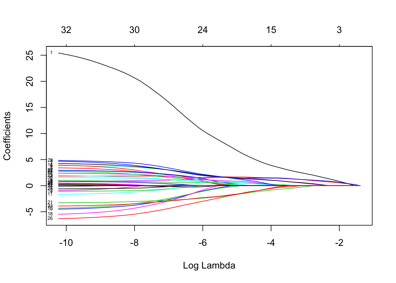
Choice of \(\lambda\) through CV
Use cv.glmnet() to get the two default choices lambda.min and lambda.1se for the lasso tuning parameter \(\lambda\) when the classification error is minimised. Calculate these two values on the log-scale as well to relate to the above lasso coefficient plot.
set.seed(1)
lasso.cv = cv.glmnet(x, y, family = "binomial", type.measure = "class")
c(lasso.cv$lambda.min, lasso.cv$lambda.1se)
## [1] 0.006614550 0.009596579round(log(c(lasso.cv$lambda.min, lasso.cv$lambda.1se)), 2)## [1] -5.02 -4.65plot(lasso.cv)
Explore how sensitive the lambda.1se value is to different choices of \(k\) in the \(k\)-fold CV (changing the default option nfolds=10) as well as to different choices of the random seed.
set.seed(2)
lasso.cv = cv.glmnet(x, y, family = "binomial", type.measure = "class",
    nfolds = 10)
round(log(lasso.cv$lambda.1se), 2)
## [1] -4lasso.cv = cv.glmnet(x, y, family = "binomial", type.measure = "class",
nfolds = 5)
round(log(lasso.cv$lambda.1se), 2)## [1] -3.72lasso.cv = cv.glmnet(x, y, family = "binomial", type.measure = "class",
nfolds = 3)
round(log(lasso.cv$lambda.1se), 2)## [1] -2.32set.seed(3)
lasso.cv = cv.glmnet(x, y, family = "binomial", type.measure = "class",
nfolds = 10)
round(log(lasso.cv$lambda.1se), 2)## [1] -5.67lasso.cv = cv.glmnet(x, y, family = "binomial", type.measure = "class",
nfolds = 5)
round(log(lasso.cv$lambda.1se), 2)## [1] -4.37lasso.cv = cv.glmnet(x, y, family = "binomial", type.measure = "class",
nfolds = 3)
round(log(lasso.cv$lambda.1se), 2)## [1] -2.6# we could take a more organised approach to assess the
# variability:
set.seed(2)
nreps = 25
lse_nfolds10 = lse_nfolds5 = lse_nfolds3 = rep(NA, nreps)
for (i in 1:nreps) {
lasso.cv = cv.glmnet(x, y, family = "binomial", type.measure = "class",
nfolds = 10)
lse_nfolds10[i] = log(lasso.cv$lambda.1se)
lasso.cv = cv.glmnet(x, y, family = "binomial", type.measure = "class",
nfolds = 5)
lse_nfolds5[i] = log(lasso.cv$lambda.1se)
lasso.cv = cv.glmnet(x, y, family = "binomial", type.measure = "class",
nfolds = 3)
lse_nfolds3[i] = log(lasso.cv$lambda.1se)
}
boxplot(lse_nfolds10, lse_nfolds5, lse_nfolds3, names = c("nfolds=10",
"nfolds=5", "nfolds=3"), ylab = "log(Lambda)")Choice of \(\lambda\) through AIC and BIC
Choose that \(\lambda\) value that gives smallest AIC and BIC for the models on the lasso path.
To calculate the \(-2\times\text{LogLik}\) for the models on the lasso path use the function deviance.glmnet (check help(deviance.glmnet)) and for calculating the number of non-zero regression parameters use the value df of the glmnet object.
Show also the corresponding regression coefficients.
length(lasso.fit$lambda)## [1] 96lasso.aic = deviance(lasso.fit) + 2 * lasso.fit$df
lasso.bic = deviance(lasso.fit) + log(351) * lasso.fit$df
which.min(lasso.aic)## [1] 64which.min(lasso.bic)## [1] 37log(lasso.fit$lambda[64])## [1] -7.251293log(lasso.fit$lambda[37])## [1] -4.739382coef(lasso.fit)[, c(37, 64)]## 34 x 2 sparse Matrix of class "dgCMatrix"
## s36 s63
## (Intercept) -7.63804244 -19.97760594
## X1 5.83649771 17.33128212
## X3 1.65355461 1.79013288
## X4 . -0.71473590
## X5 1.48511903 3.24988608
## X6 0.92605010 3.17590149
## X7 1.43732303 1.02380148
## X8 1.32579242 3.20339882
## X9 . 2.28104503
## X10 0.45782632 0.68954585
## X11 . -2.99786770
## X12 . -0.83889824
## X13 . .
## X14 . 0.03278883
## X15 . 2.30522823
## X16 . -2.74363799
## X17 . 0.43751730
## X18 0.45803345 2.13217256
## X19 . -3.35870761
## X20 . .
## X21 . .
## X22 -1.43984206 -2.85916411
## X23 0.08460504 2.31187561
## X24 0.12849989 1.30783045
## X25 0.72605376 1.89735684
## X26 . -0.27175033
## X27 -1.29590306 -4.69533343
## X28 . .
## X29 . 1.73637193
## X30 1.09798231 3.67431267
## X31 0.52476560 1.23671045
## X32 . .
## X33 . -0.12089348
## X34 -1.34765320 -3.09040097Maximum-likelihood, ridge, lasso and elastic-net
Visualise the parameter estimates from the maximum-likelihood (ML), lasso, ridge and elastic-net methods. When obtaining the parameter estimates, use lambda.1se for each of the three regularization methods. Recall that glm fits logistic regression models with ML.
dat2 = dat[, -2]
dat2$y = as.numeric(dat2$y) - 1
b.ml = coef(glm(y ~ ., family = binomial(link = "logit"), data = dat2))[-1]
set.seed(4)
cv.glmnet(x, y, family = "binomial", type.measure = "class",
    alpha = 0)$lambda.1se
## [1] 0.1005353b.ridge = coef(glmnet(x, y, family = "binomial", alpha = 0, lambda = 0.1))[-1]
cv.glmnet(x, y, family = "binomial", type.measure = "class",
alpha = 0.5)$lambda.1se## [1] 0.03681076b.enet = coef(glmnet(x, y, family = "binomial", alpha = 0.5,
lambda = 0.037))[-1]
cv.glmnet(x, y, family = "binomial", type.measure = "class")$lambda.1se## [1] 0.04251881b.lasso = coef(glmnet(x, y, family = "binomial", lambda = 0.043))[-1]
B = cbind(b.ml, b.ridge, b.enet, b.lasso)
plot(1:4, B[1, ], type = "b", lty = 2, col = c(1, 2, 4, 6), ylab = "Coefficients",
xlim = c(0.75, 4.25), ylim = c(-7, 7), xlab = "")
for (i in 2:32) {
points(1:4, B[i, ], type = "b", lty = 2, col = c(1, 2, 4,
6))
}
text(1, 6.2, "ML")
text(2, -3, "Ridge", col = 2)
text(3, 5, "Elastic-net", col = 4)
text(4, -3, "Lasso", col = 6)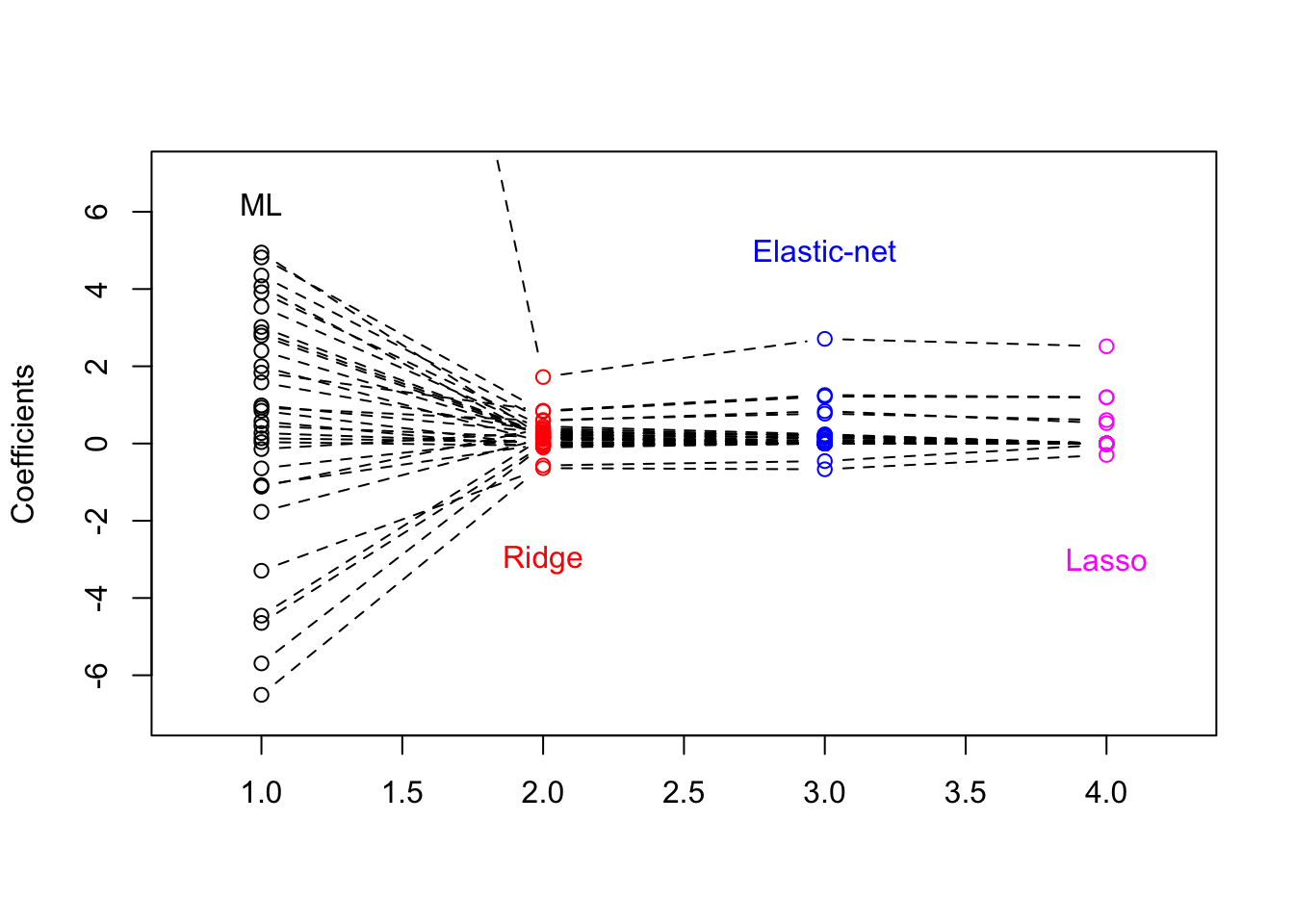
Which is better, lasso, ridge or elastic-net?
It is impossible to know for real data what classifier (regression model) will do best and often it is not even clear what is meant by ‘best’. We are going to use again the classification error, but this time of independent data to assess what is ‘best’ in terms of prediction.
To empirically determine this prediction error, a standard approach is to split the data into a training set (often around 2/3 of the observations) and into a validation set (the remaining observations).
Produce such a random split:
n = length(y)
n
## [1] 351set.seed(2015)
train = sample(1:n, 2 * n/3) # by default replace=FALSE in sample()
length(train)/n## [1] 0.6666667max(table(train)) # if 1, then no ties in the sampled observations## [1] 1test = (1:n)[-train]- Calculate the validation classification error rate for the lasso when the logistic regression model is based on the training sample and \(\lambda\) is selected through
lambda.minfromcv.glmnet.
lasso.cv = cv.glmnet(x[train, ], y[train], family = "binomial",
    type.measure = "class")
lasso.fit = glmnet(x[train, ], y[train], family = "binomial")
# calculate predicted probability to be 'g' - second level of
# categorical y - through type='response'
lasso.predict.prob = predict(lasso.fit, s = lasso.cv$lambda.min,
    newx = x[test, ], type = "response")  # check help(predict.glmnet)
predict.g = lasso.predict.prob > 0.5
table(y[test], predict.g)
## predict.g
## FALSE TRUE
## b 36 8
## g 6 67sum(table(y[test], predict.g)[c(2, 3)])/length(test)## [1] 0.1196581# calculate predicted y through type='class'
lasso.predict.y = predict(lasso.fit, s = lasso.cv$lambda.min,
newx = x[test, ], type = "class") # check help(predict.glmnet)
mean(lasso.predict.y != y[test])## [1] 0.1196581- Calculate the validation classification error rate for the elastic-net (with \(\alpha=0.5\)) and ridge regression as well.
enet.cv = cv.glmnet(x[train, ], y[train], family = "binomial",
    type.measure = "class", alpha = 0.5)
enet.fit = glmnet(x[train, ], y[train], family = "binomial",
    alpha = 0.5)
enet.predict.y = predict(enet.fit, s = enet.cv$lambda.min, newx = x[test,
    ], type = "class")
mean(enet.predict.y != y[test])
## [1] 0.1111111ridge.cv = cv.glmnet(x[train, ], y[train], family = "binomial",
type.measure = "class", alpha = 0)
ridge.fit = glmnet(x[train, ], y[train], family = "binomial",
alpha = 0)
ridge.predict.y = predict(ridge.fit, s = ridge.cv$lambda.min,
newx = x[test, ], type = "class")
mean(ridge.predict.y != y[test])## [1] 0.1538462Simulation study
To explore the performance of the above regularization methods in normal linear regression when \(1000 = p > n = 300\) let us consider a true model \[ \boldsymbol{y} = \boldsymbol{X}\boldsymbol{\beta} + \boldsymbol{\epsilon} \quad\text{with}\quad \boldsymbol{\epsilon} \sim N(\boldsymbol{0},\boldsymbol{I}) \]
Setting 1
- Sparse signal, 1% non-zero regression parameters
- Predictors have small empirical correlations
Generate the regression data
set.seed(300)
n = 300
p = 1000
p.nonzero = 10
x = matrix(rnorm(n * p), nrow = n, ncol = p)
b.nonzero = rexp(p.nonzero) * (sign(rnorm(p.nonzero)))
b.nonzero
## [1] -2.3780961 0.3871070 0.7883509 0.1876987 1.3820593
## [6] 0.0685901 2.1213078 0.3013759 -0.4809320 -0.9830124beta = c(b.nonzero, rep(0, p - p.nonzero))
y = x %*% beta + rnorm(n)Split the data into a 2/3 training and 1/3 test set as before.
train = sample(1:n, 2 * n/3)
x.train = x[train, ]
x.test = x[-train, ]
y.train = y[train]
y.test = y[-train]- Fit the lasso, elastic-net (with \(\alpha=0.5\)) and ridge regression.
lasso.fit = glmnet(x.train, y.train, family = "gaussian", alpha = 1)
ridge.fit = glmnet(x.train, y.train, family = "gaussian", alpha = 0)
enet.fit = glmnet(x.train, y.train, family = "gaussian", alpha = 0.5)- Write a loop, varying \(\alpha\) from \(0,0.1,\ldots 1\) and extract
mse(mean squared error) fromcv.glmnetfor 10-fold CV. Plot the solution paths and cross-validated MSE as function of \(\lambda\).
fit = list()
for (i in 0:10) {
    fit[[i + 1]] = cv.glmnet(x.train, y.train, type.measure = "mse",
        alpha = i/10, family = "gaussian")
}
names(fit) = 0:10

par(mfrow = c(3, 2))
plot(lasso.fit, xvar = "lambda")
plot(fit[["10"]], main = "lasso")

plot(ridge.fit, xvar = "lambda")
plot(fit[["5"]], main = "elastic-net")

plot(enet.fit, xvar = "lambda")
plot(fit[["0"]], main = "ridge")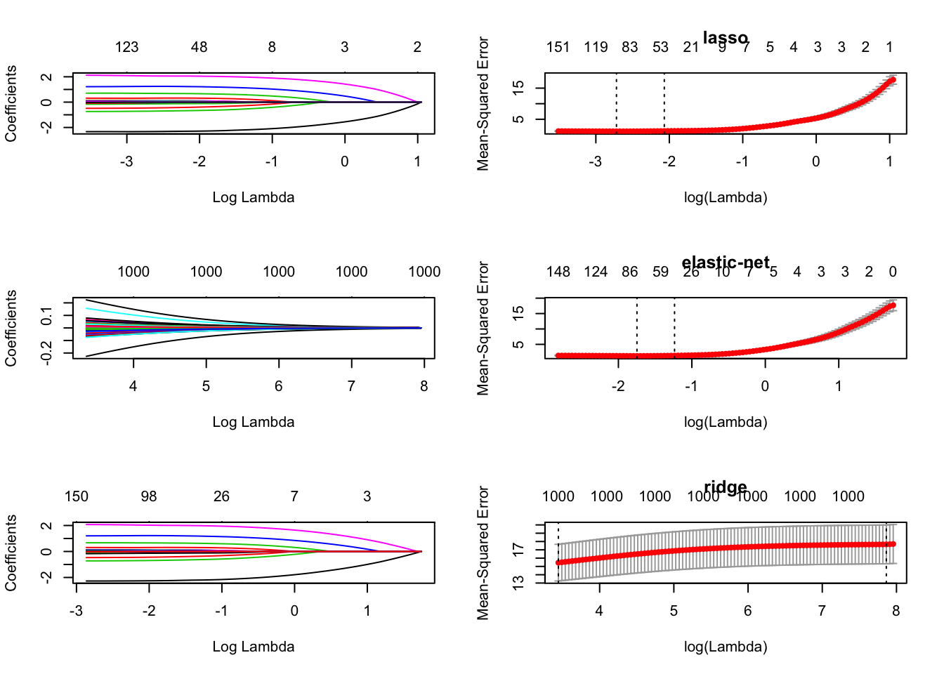
- Calculate the MSE on the test set.
yhat0 = predict(fit[["0"]], s = fit[["0"]]$lambda.1se, newx = x.test)
yhat1 = predict(fit[["1"]], s = fit[["1"]]$lambda.1se, newx = x.test)
yhat2 = predict(fit[["2"]], s = fit[["2"]]$lambda.1se, newx = x.test)
yhat3 = predict(fit[["3"]], s = fit[["3"]]$lambda.1se, newx = x.test)
yhat4 = predict(fit[["4"]], s = fit[["4"]]$lambda.1se, newx = x.test)
yhat5 = predict(fit[["5"]], s = fit[["5"]]$lambda.1se, newx = x.test)
yhat6 = predict(fit[["6"]], s = fit[["6"]]$lambda.1se, newx = x.test)
yhat7 = predict(fit[["7"]], s = fit[["7"]]$lambda.1se, newx = x.test)
yhat8 = predict(fit[["8"]], s = fit[["8"]]$lambda.1se, newx = x.test)
yhat9 = predict(fit[["9"]], s = fit[["9"]]$lambda.1se, newx = x.test)
yhat10 = predict(fit[["10"]], s = fit[["10"]]$lambda.1se, newx = x.test)

mse0 = mean((y.test - yhat0)^2)
mse1 = mean((y.test - yhat1)^2)
mse2 = mean((y.test - yhat2)^2)
mse3 = mean((y.test - yhat3)^2)
mse4 = mean((y.test - yhat4)^2)
mse5 = mean((y.test - yhat5)^2)
mse6 = mean((y.test - yhat6)^2)
mse7 = mean((y.test - yhat7)^2)
mse8 = mean((y.test - yhat8)^2)
mse9 = mean((y.test - yhat9)^2)
mse10 = mean((y.test - yhat10)^2)
c(mse0, mse1, mse2, mse3, mse4, mse5, mse6, mse7, mse8, mse9,
    mse10)
## [1] 15.445985 3.432268 2.228483 1.929294 1.829045
## [6] 1.739102 1.691122 1.661092 1.646961 1.626372
## [11] 1.619253Here, lasso has smallest MSE and we note that lasso seems to do well when there are lots of redundant variables.
Setting 2
- Non-sparse signal, \(n/p\) non-zero regression parameters
- Predictors have small empirical correlations
Generate the regression data
set.seed(300)
n = 300
p = 1000
p.nonzero = n
x = matrix(rnorm(n * p), nrow = n, ncol = p)
b.nonzero = rexp(p.nonzero) * (sign(rnorm(p.nonzero)))
summary(b.nonzero)
## Min. 1st Qu. Median Mean 3rd Qu. Max.
## -5.59419 -0.68859 0.01699 0.03362 0.76344 3.70905beta = c(b.nonzero, rep(0, p - p.nonzero))
y = x %*% beta + rnorm(n)Split the data into a 2/3 training and 1/3 test set as before.
train = sample(1:n, 2 * n/3)
x.train = x[train, ]
x.test = x[-train, ]
y.train = y[train]
y.test = y[-train]- Fit the lasso, elastic-net (with \(\alpha=0.5\)) and ridge regression.
lasso.fit = glmnet(x.train, y.train, family = "gaussian", alpha = 1)
ridge.fit = glmnet(x.train, y.train, family = "gaussian", alpha = 0)
enet.fit = glmnet(x.train, y.train, family = "gaussian", alpha = 0.5)- Write a loop, varying \(\alpha\) from \(0,0.1,\ldots 1\) and extract
mse(mean squared error) fromcv.glmnetfor 10-fold CV.
for (i in 0:10) {
    assign(paste("fit", i, sep = ""), cv.glmnet(x.train, y.train,
        type.measure = "mse", alpha = i/10, family = "gaussian"))
}- Plot the solution paths and cross-validated MSE as function of \(\lambda\).
par(mfrow = c(3, 2))
plot(lasso.fit, xvar = "lambda")
plot(fit10, main = "lasso")

plot(ridge.fit, xvar = "lambda")
plot(fit5, main = "elastic-net")

plot(enet.fit, xvar = "lambda")
plot(fit0, main = "ridge")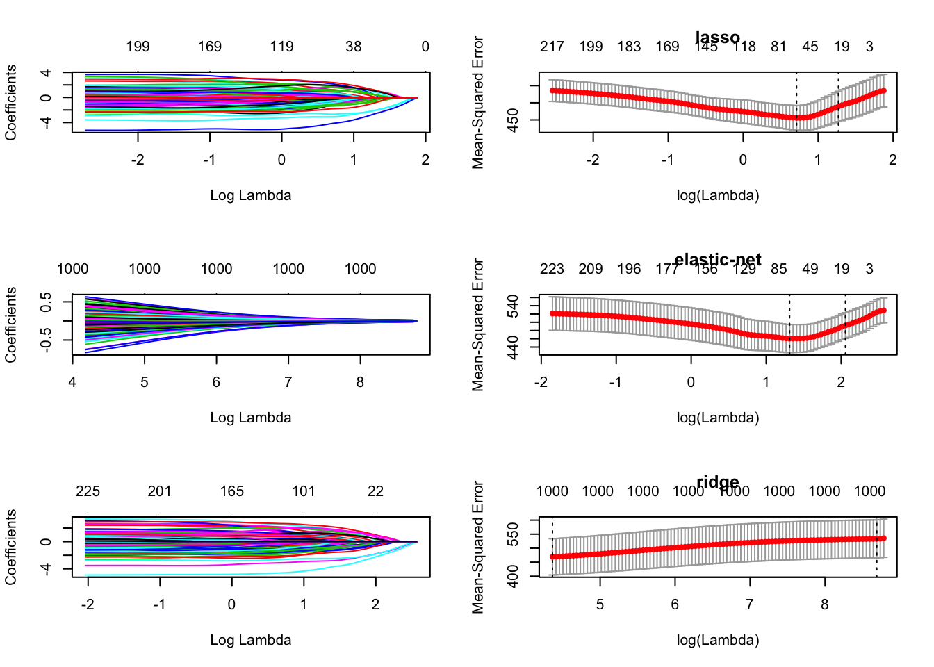
- Calculate the MSE on the test set.
yhat0 = predict(fit0, s = fit0$lambda.1se, newx = x.test)
yhat1 = predict(fit1, s = fit1$lambda.1se, newx = x.test)
yhat2 = predict(fit2, s = fit2$lambda.1se, newx = x.test)
yhat3 = predict(fit3, s = fit3$lambda.1se, newx = x.test)
yhat4 = predict(fit4, s = fit4$lambda.1se, newx = x.test)
yhat5 = predict(fit5, s = fit5$lambda.1se, newx = x.test)
yhat6 = predict(fit6, s = fit6$lambda.1se, newx = x.test)
yhat7 = predict(fit7, s = fit7$lambda.1se, newx = x.test)
yhat8 = predict(fit8, s = fit8$lambda.1se, newx = x.test)
yhat9 = predict(fit9, s = fit9$lambda.1se, newx = x.test)
yhat10 = predict(fit10, s = fit10$lambda.1se, newx = x.test)

mse0 = mean((y.test - yhat0)^2)
mse1 = mean((y.test - yhat1)^2)
mse2 = mean((y.test - yhat2)^2)
mse3 = mean((y.test - yhat3)^2)
mse4 = mean((y.test - yhat4)^2)
mse5 = mean((y.test - yhat5)^2)
mse6 = mean((y.test - yhat6)^2)
mse7 = mean((y.test - yhat7)^2)
mse8 = mean((y.test - yhat8)^2)
mse9 = mean((y.test - yhat9)^2)
mse10 = mean((y.test - yhat10)^2)
c(mse0, mse1, mse2, mse3, mse4, mse5, mse6, mse7, mse8, mse9,
    mse10)
## [1] 371.7866 328.3805 310.3128 349.3736 316.7003 332.5072
## [7] 319.3968 343.8416 304.7279 309.7283 315.9038Here, elastic-net has smallest MSE but we note that the MSE is much more variable (as \(\alpha\) is varied).
Additional settings
Investigate effect of correlated columns in \(\boldsymbol{X}\), for example \(\text{Cov}(\boldsymbol{X})_{ij}=(0.9)^{|i−j|}\).
n = 100
p = 60
CovMatrix = outer(1:p, 1:p, function(x, y) {
    0.9^abs(x - y)
})
x = MASS::mvrnorm(n, rep(0, p), CovMatrix)
Similar setupas above but different ways to generate non-zero regression coefficients
- All are equal to 1
- Some are large (say 4), intermediate (1) and small (0.25)