Lab 2: Exhaustive searching and GLMs

Crime data

Birthweight data

Rock-wallabies: cross validation

Advanced: Stagewise selection

Learning outcomes

Marginality principle
Exhaustive search for linear models
Exhaustive search for generalised linear models

Required R packages:

install.packages(c("mplot", "leaps", "bestglm", "car"))

Crime data

data("UScrime", package = "MASS")
M0 = lm(y ~ 1, data = UScrime)  # Null model
M1 = lm(y ~ ., data = UScrime)  # Full model

Exercises

Use the regsubsets() function from the leaps package to obtain the 50 best models for each model size and plot their RSS against model dimension.

library(leaps)
rgsbst.out = regsubsets(y ~ ., data = UScrime, nbest = 50, nvmax = NULL, 
    method = "exhaustive", really.big = TRUE)
rss = summary(rgsbst.out)$rss
p = rowSums(summary(rgsbst.out)$which)
plot(rss ~ p)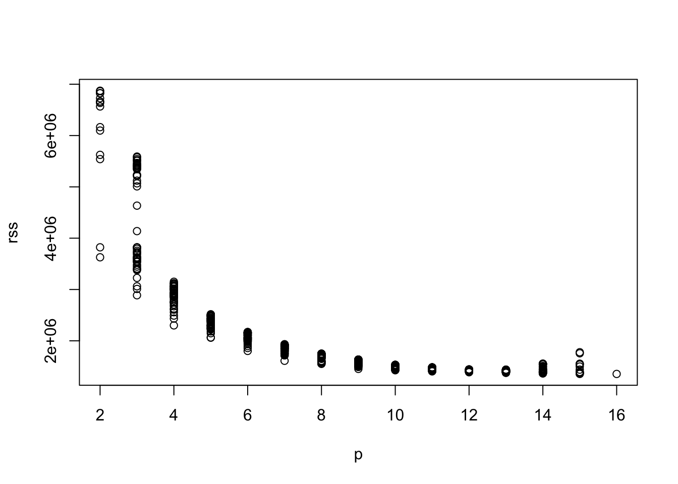

Use the method = "forward" and method = "backward" and method = "exhaustive" options to perform forward, backward and exhaustive model selection and compare the results (only find a single best model at each dimension). Hint: The regsubsets function returns several information criteria, choose for example Mallow’s Cp.

fwd = regsubsets(y ~ ., data = UScrime, nvmax = NULL, method = "forward")
bwd = regsubsets(y ~ ., data = UScrime, nvmax = NULL, method = "backward")
exh = regsubsets(y ~ ., data = UScrime, nvmax = NULL, method = "exhaustive")
as.data.frame(summary(fwd)$outmat)

##           M So Ed Po1 Po2 LF M.F Pop NW U1 U2 GDP Ineq Prob
## 1  ( 1 )            *                                      
## 2  ( 1 )            *                                *     
## 3  ( 1 )        *   *                                *     
## 4  ( 1 )  *     *   *                                *     
## 5  ( 1 )  *     *   *                                *    *
## 6  ( 1 )  *     *   *                       *        *    *
## 7  ( 1 )  *     *   *                       *   *    *    *
## 8  ( 1 )  *     *   *              *        *   *    *    *
## 9  ( 1 )  *     *   *              *     *  *   *    *    *
## 10  ( 1 ) *     *   *          *   *     *  *   *    *    *
## 11  ( 1 ) *     *   *   *      *   *     *  *   *    *    *
## 12  ( 1 ) *     *   *   *      *   *  *  *  *   *    *    *
## 13  ( 1 ) *     *   *   *  *   *   *  *  *  *   *    *    *
## 14  ( 1 ) *     *   *   *  *   *   *  *  *  *   *    *    *
## 15  ( 1 ) *  *  *   *   *  *   *   *  *  *  *   *    *    *
##           Time
## 1  ( 1 )      
## 2  ( 1 )      
## 3  ( 1 )      
## 4  ( 1 )      
## 5  ( 1 )      
## 6  ( 1 )      
## 7  ( 1 )      
## 8  ( 1 )      
## 9  ( 1 )      
## 10  ( 1 )     
## 11  ( 1 )     
## 12  ( 1 )     
## 13  ( 1 )     
## 14  ( 1 )    *
## 15  ( 1 )    *

as.data.frame(summary(bwd)$outmat)

##           M So Ed Po1 Po2 LF M.F Pop NW U1 U2 GDP Ineq Prob
## 1  ( 1 )            *                                      
## 2  ( 1 )            *                                *     
## 3  ( 1 )        *   *                                *     
## 4  ( 1 )  *     *   *                                *     
## 5  ( 1 )  *     *   *                                *    *
## 6  ( 1 )  *     *   *                       *        *    *
## 7  ( 1 )  *     *   *                    *  *        *    *
## 8  ( 1 )  *     *   *          *         *  *        *    *
## 9  ( 1 )  *     *   *          *         *  *   *    *    *
## 10  ( 1 ) *     *   *          *   *     *  *   *    *    *
## 11  ( 1 ) *     *   *   *      *   *     *  *   *    *    *
## 12  ( 1 ) *     *   *   *      *   *  *  *  *   *    *    *
## 13  ( 1 ) *     *   *   *  *   *   *  *  *  *   *    *    *
## 14  ( 1 ) *     *   *   *  *   *   *  *  *  *   *    *    *
## 15  ( 1 ) *  *  *   *   *  *   *   *  *  *  *   *    *    *
##           Time
## 1  ( 1 )      
## 2  ( 1 )      
## 3  ( 1 )      
## 4  ( 1 )      
## 5  ( 1 )      
## 6  ( 1 )      
## 7  ( 1 )      
## 8  ( 1 )      
## 9  ( 1 )      
## 10  ( 1 )     
## 11  ( 1 )     
## 12  ( 1 )     
## 13  ( 1 )     
## 14  ( 1 )    *
## 15  ( 1 )    *

par(mar = c(4.5, 4.5, 1, 1), mfrow = c(1, 1))
plot(summary(fwd)$cp, col = "blue", type = "l", xlab = "Model size", 
    ylab = "Cp")
lines(summary(bwd)$cp, col = "red")
lines(summary(exh)$cp, col = "orange")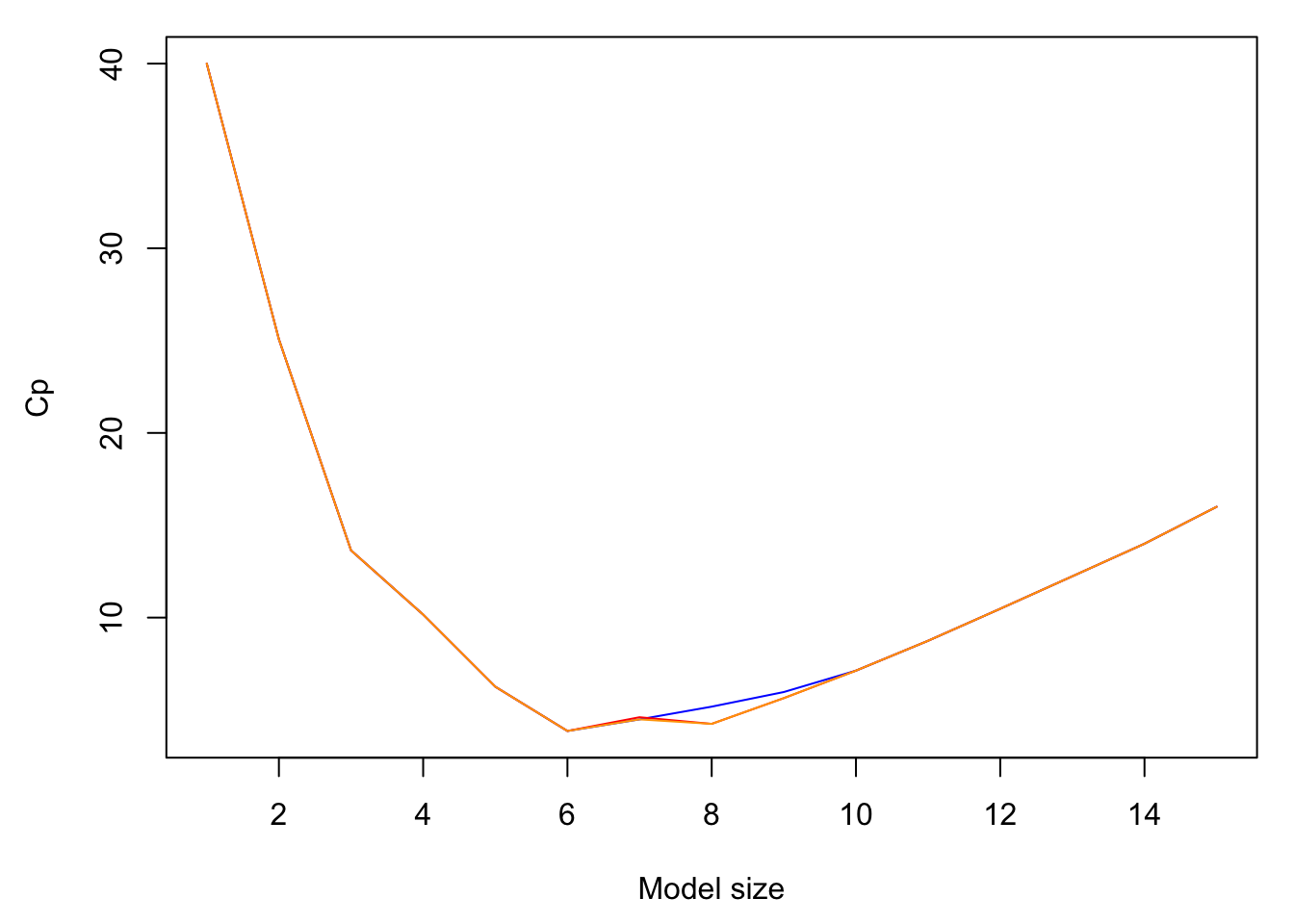

# They haven't always selected identical models along the
# path, though in this instance they both found the model
# that minimised the overall Cp (confirmed through an
# exhaustive search).

Use the plot method associated with regsubsets objects to visualise the BIC for the various models identified.

par(mfrow = c(3, 1))
plot(fwd, main = "Forward")
plot(bwd, main = "Backward")
plot(exh, main = "Exhaustive")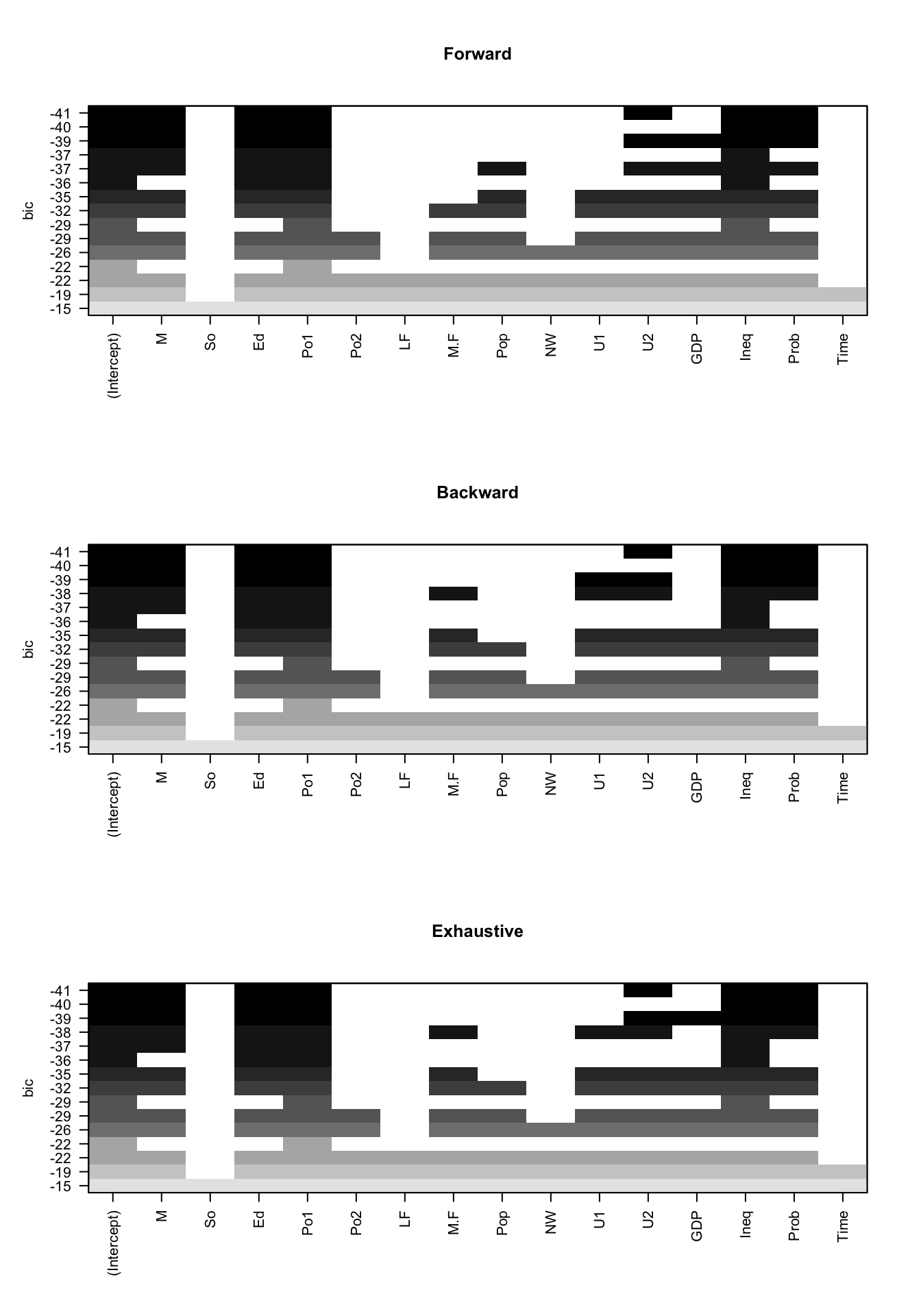

# To have a different criterion on the y-axis in the plots
# specify scale=c('bic', 'Cp', 'adjr2', 'r2') in plot()

The car package offers alternative plot methods to visualise the results from a call to regsubsets(). The code below plots $C_p$ against dimension for a regsubsets object called exh. Try plotting adjusted $R^2$ against dimension.

library(car)

## Loading required package: carData

par(mar = c(4.5, 4.5, 1, 1), mfrow = c(1, 1))
subsets(exh, statistic = "cp", legend = FALSE, max.size = 8)

##      Abbreviation
## M               M
## So              S
## Ed              E
## Po1            P1
## Po2            P2
## LF              L
## M.F            M.
## Pop            Pp
## NW              N
## U1             U1
## U2             U2
## GDP             G
## Ineq            I
## Prob           Pr
## Time            T

abline(a = 0, b = 1, lty = 2)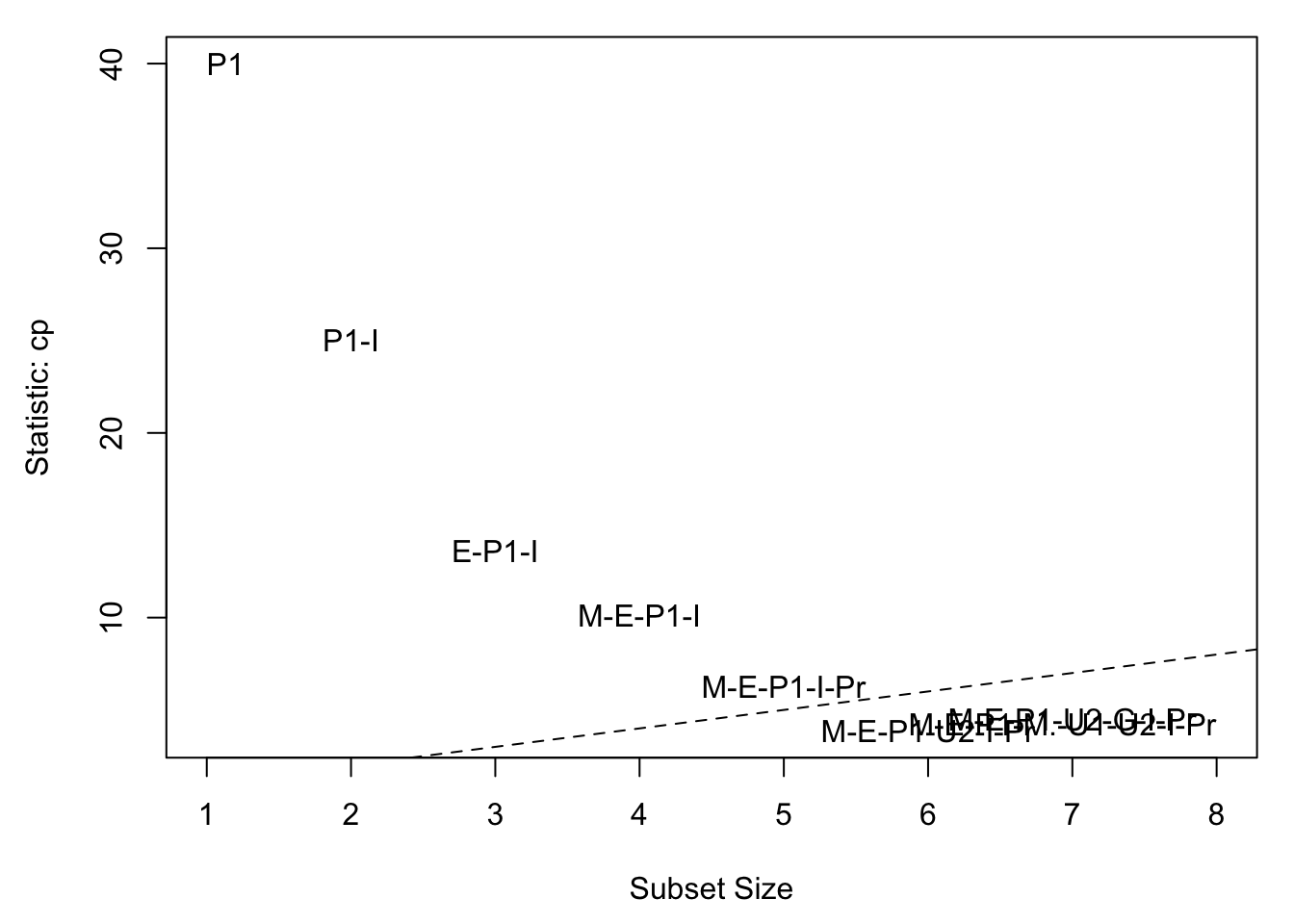

subsets(exh, statistic = "adjr2", legend = FALSE, max.size = 10)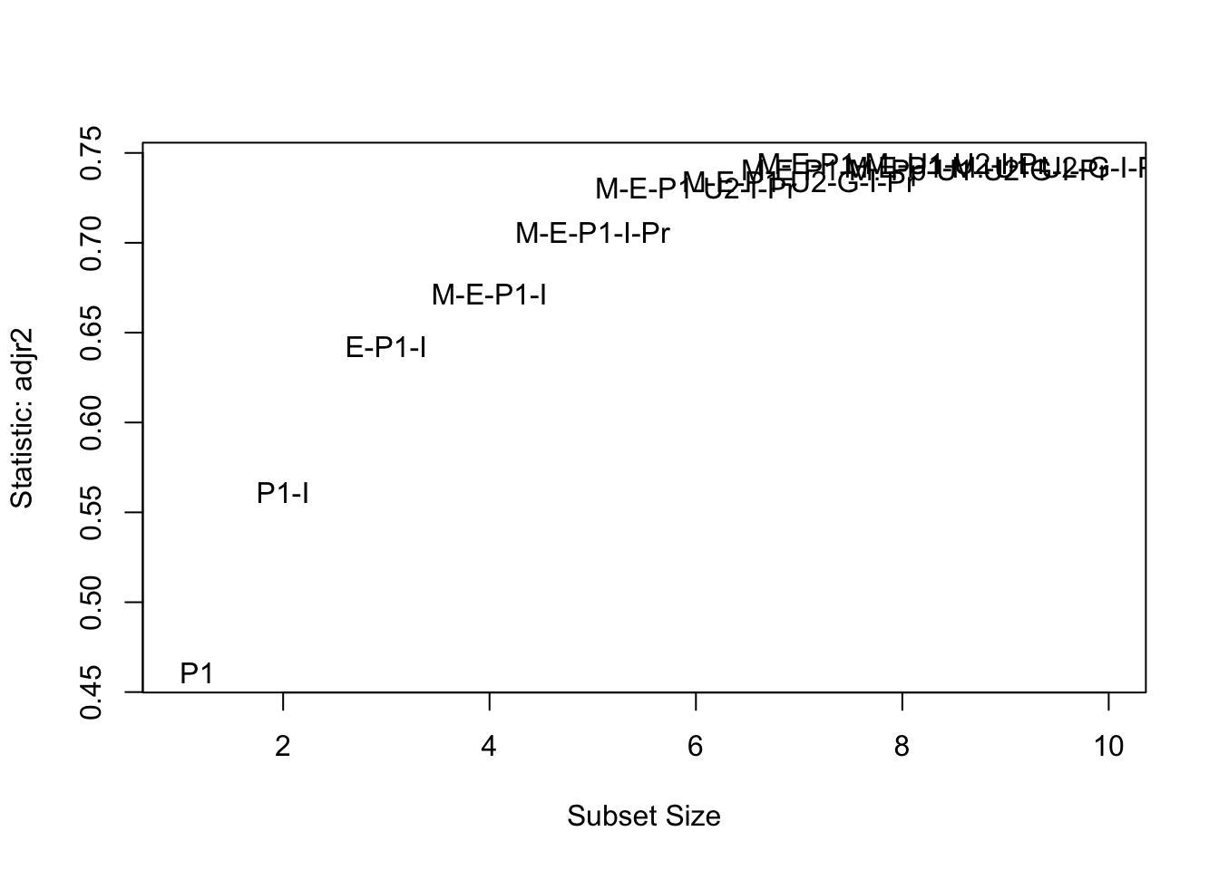

##      Abbreviation
## M               M
## So              S
## Ed              E
## Po1            P1
## Po2            P2
## LF              L
## M.F            M.
## Pop            Pp
## NW              N
## U1             U1
## U2             U2
## GDP             G
## Ineq            I
## Prob           Pr
## Time            T

Birthweight data

The second example is the birthwt dataset from the MASS package which has data on 189 births at the Baystate Medical Centre, Springfield, Massachusetts during 1986 (Venables and Ripley, 2002) The main variable of interest is low birth weight, a binary response variable low (Hosmer and Lemeshow, 1989). Take the same approach to modelling the full model as in Venables and Ripley (2002), where ptl is reduced to a binary indicator of past history and ftv is reduced to a factor with three levels:

library(MASS)
bwt <- with(birthwt, {
    race <- factor(race, labels = c("white", "black", "other"))
    ptd <- factor(ptl > 0)
    ftv <- factor(ftv)
    levels(ftv)[-(1:2)] <- "2+"
    data.frame(low = factor(low), age, lwt, race, smoke = (smoke > 
        0), ptd, ht = (ht > 0), ui = (ui > 0), ftv)
})
options(contrasts = c("contr.treatment", "contr.poly"))
bw.glm1 <- glm(low ~ ., family = binomial, data = bwt)
bw.glm0 <- glm(low ~ 1, family = binomial, data = bwt)
summary(bw.glm1)

## 
## Call:
## glm(formula = low ~ ., family = binomial, data = bwt)
## 
## Deviance Residuals: 
##     Min       1Q   Median       3Q      Max  
## -1.7038  -0.8068  -0.5008   0.8835   2.2152  
## 
## Coefficients:
##             Estimate Std. Error z value Pr(>|z|)   
## (Intercept)  0.82302    1.24471   0.661  0.50848   
## age         -0.03723    0.03870  -0.962  0.33602   
## lwt         -0.01565    0.00708  -2.211  0.02705 * 
## raceblack    1.19241    0.53597   2.225  0.02609 * 
## raceother    0.74069    0.46174   1.604  0.10869   
## smokeTRUE    0.75553    0.42502   1.778  0.07546 . 
## ptdTRUE      1.34376    0.48062   2.796  0.00518 **
## htTRUE       1.91317    0.72074   2.654  0.00794 **
## uiTRUE       0.68019    0.46434   1.465  0.14296   
## ftv1        -0.43638    0.47939  -0.910  0.36268   
## ftv2+        0.17901    0.45638   0.392  0.69488   
## ---
## Signif. codes:  
## 0 '***' 0.001 '**' 0.01 '*' 0.05 '.' 0.1 ' ' 1
## 
## (Dispersion parameter for binomial family taken to be 1)
## 
##     Null deviance: 234.67  on 188  degrees of freedom
## Residual deviance: 195.48  on 178  degrees of freedom
## AIC: 217.48
## 
## Number of Fisher Scoring iterations: 4

Exercises

Use forward and backward stepwise to identify potential models. Do you get the same model using both approaches?

step(bw.glm1)

## Start:  AIC=217.48
## low ~ age + lwt + race + smoke + ptd + ht + ui + ftv
## 
##         Df Deviance    AIC
## - ftv    2   196.83 214.83
## - age    1   196.42 216.42
## <none>       195.48 217.48
## - ui     1   197.59 217.59
## - smoke  1   198.67 218.67
## - race   2   201.23 219.23
## - lwt    1   200.95 220.95
## - ht     1   202.93 222.93
## - ptd    1   203.58 223.58
## 
## Step:  AIC=214.83
## low ~ age + lwt + race + smoke + ptd + ht + ui
## 
##         Df Deviance    AIC
## - age    1   197.85 213.85
## <none>       196.83 214.83
## - ui     1   199.15 215.15
## - race   2   203.24 217.24
## - smoke  1   201.25 217.25
## - lwt    1   201.83 217.83
## - ptd    1   203.95 219.95
## - ht     1   204.01 220.01
## 
## Step:  AIC=213.85
## low ~ lwt + race + smoke + ptd + ht + ui
## 
##         Df Deviance    AIC
## <none>       197.85 213.85
## - ui     1   200.48 214.48
## - smoke  1   202.57 216.57
## - race   2   205.47 217.47
## - lwt    1   203.82 217.82
## - ptd    1   204.22 218.22
## - ht     1   205.16 219.16

## 
## Call:  glm(formula = low ~ lwt + race + smoke + ptd + ht + ui, family = binomial, 
##     data = bwt)
## 
## Coefficients:
## (Intercept)          lwt    raceblack    raceother  
##    -0.12533     -0.01592      1.30086      0.85441  
##   smokeTRUE      ptdTRUE       htTRUE       uiTRUE  
##     0.86658      1.12886      1.86690      0.75065  
## 
## Degrees of Freedom: 188 Total (i.e. Null);  181 Residual
## Null Deviance:       234.7 
## Residual Deviance: 197.9     AIC: 213.9

step(bw.glm0, scope = list(upper = bw.glm1, lower = bw.glm0), 
    method = "forward")

## Start:  AIC=236.67
## low ~ 1
## 
##         Df Deviance    AIC
## + ptd    1   221.90 225.90
## + lwt    1   228.69 232.69
## + ui     1   229.60 233.60
## + smoke  1   229.81 233.81
## + ht     1   230.65 234.65
## + race   2   229.66 235.66
## + age    1   231.91 235.91
## <none>       234.67 236.67
## + ftv    2   232.09 238.09
## 
## Step:  AIC=225.9
## low ~ ptd
## 
##         Df Deviance    AIC
## + age    1   217.30 223.30
## + lwt    1   217.50 223.50
## + ht     1   217.66 223.66
## + race   2   217.02 225.02
## + ui     1   219.12 225.12
## + smoke  1   219.33 225.33
## + ftv    2   217.88 225.88
## <none>       221.90 225.90
## - ptd    1   234.67 236.67
## 
## Step:  AIC=223.3
## low ~ ptd + age
## 
##         Df Deviance    AIC
## + ht     1   213.12 221.12
## + lwt    1   214.31 222.31
## + smoke  1   215.04 223.04
## + ui     1   215.13 223.13
## <none>       217.30 223.30
## + race   2   213.97 223.97
## + ftv    2   214.63 224.63
## - age    1   221.90 225.90
## - ptd    1   231.91 235.91
## 
## Step:  AIC=221.12
## low ~ ptd + age + ht
## 
##         Df Deviance    AIC
## + lwt    1   207.43 217.43
## + ui     1   210.13 220.13
## + smoke  1   210.89 220.89
## <none>       213.12 221.12
## + race   2   210.06 222.06
## + ftv    2   210.38 222.38
## - ht     1   217.30 223.30
## - age    1   217.66 223.66
## - ptd    1   227.93 233.93
## 
## Step:  AIC=217.43
## low ~ ptd + age + ht + lwt
## 
##         Df Deviance    AIC
## + ui     1   205.15 217.15
## + smoke  1   205.39 217.39
## <none>       207.43 217.43
## + race   2   203.77 217.77
## - age    1   210.12 218.12
## + ftv    2   204.33 218.33
## - lwt    1   213.12 221.12
## - ht     1   214.31 222.31
## - ptd    1   219.88 227.88
## 
## Step:  AIC=217.15
## low ~ ptd + age + ht + lwt + ui
## 
##         Df Deviance    AIC
## <none>       205.15 217.15
## + smoke  1   203.24 217.24
## + race   2   201.25 217.25
## - ui     1   207.43 217.43
## - age    1   207.51 217.51
## + ftv    2   202.41 218.41
## - lwt    1   210.13 220.13
## - ht     1   212.70 222.70
## - ptd    1   215.48 225.48

## 
## Call:  glm(formula = low ~ ptd + age + ht + lwt + ui, family = binomial, 
##     data = bwt)
## 
## Coefficients:
## (Intercept)      ptdTRUE          age       htTRUE  
##     1.74560      1.42123     -0.05331      1.90580  
##         lwt       uiTRUE  
##    -0.01437      0.69193  
## 
## Degrees of Freedom: 188 Total (i.e. Null);  183 Residual
## Null Deviance:       234.7 
## Residual Deviance: 205.2     AIC: 217.2

Use the bestglm() function from the bestglm package to identify the top 10 models according to the AIC.

library(bestglm)
# the Xy matrix needs y as the right-most variable:
bwt.Xy = bwt[, -1]
bwt.Xy = cbind(bwt.Xy, low = bwt$low)
bglm.AIC = bestglm(Xy = bwt.Xy, family = binomial, IC = "AIC", 
    TopModels = 10)

## Morgan-Tatar search since family is non-gaussian.
## Note: factors present with more than 2 levels.

bglm.AIC$BestModels

##      age  lwt  race smoke  ptd   ht    ui   ftv Criterion
## 1  FALSE TRUE  TRUE  TRUE TRUE TRUE  TRUE FALSE  211.8516
## 2  FALSE TRUE  TRUE  TRUE TRUE TRUE FALSE FALSE  212.4823
## 3   TRUE TRUE  TRUE  TRUE TRUE TRUE  TRUE FALSE  212.8337
## 4   TRUE TRUE  TRUE  TRUE TRUE TRUE FALSE FALSE  213.1514
## 5  FALSE TRUE  TRUE  TRUE TRUE TRUE  TRUE  TRUE  214.4174
## 6  FALSE TRUE  TRUE FALSE TRUE TRUE  TRUE FALSE  214.5666
## 7  FALSE TRUE  TRUE  TRUE TRUE TRUE FALSE  TRUE  214.7772
## 8   TRUE TRUE FALSE FALSE TRUE TRUE  TRUE FALSE  215.1535
## 9   TRUE TRUE FALSE  TRUE TRUE TRUE  TRUE FALSE  215.2403
## 10  TRUE TRUE  TRUE FALSE TRUE TRUE  TRUE FALSE  215.2470

summary(bglm.AIC$BestModel)

## 
## Call:
## glm(formula = y ~ ., family = family, data = Xi, weights = weights)
## 
## Deviance Residuals: 
##     Min       1Q   Median       3Q      Max  
## -1.7308  -0.7841  -0.5144   0.9539   2.1980  
## 
## Coefficients:
##              Estimate Std. Error z value Pr(>|z|)   
## (Intercept) -0.125326   0.967561  -0.130  0.89694   
## lwt         -0.015918   0.006954  -2.289  0.02207 * 
## raceblack    1.300856   0.528484   2.461  0.01384 * 
## raceother    0.854414   0.440907   1.938  0.05264 . 
## smokeTRUE    0.866582   0.404469   2.143  0.03215 * 
## ptdTRUE      1.128857   0.450388   2.506  0.01220 * 
## htTRUE       1.866895   0.707373   2.639  0.00831 **
## uiTRUE       0.750649   0.458815   1.636  0.10183   
## ---
## Signif. codes:  
## 0 '***' 0.001 '**' 0.01 '*' 0.05 '.' 0.1 ' ' 1
## 
## (Dispersion parameter for binomial family taken to be 1)
## 
##     Null deviance: 234.67  on 188  degrees of freedom
## Residual deviance: 197.85  on 181  degrees of freedom
## AIC: 213.85
## 
## Number of Fisher Scoring iterations: 4

Rock-wallabies: cross validation

Use the cross-validation argument in bestglm to identify the best rock-wallaby model using cross-validation.

data("wallabies", package = "mplot")
names(wallabies)

## [1] "rw"       "edible"   "inedible" "canopy"   "distance"
## [6] "shelter"  "lat"      "long"

wdat = data.frame(subset(wallabies, select = -c(lat, long)), 
    EaD = wallabies$edible * wallabies$distance, EaS = wallabies$edible * 
        wallabies$shelter, DaS = wallabies$distance * wallabies$shelter)
X = subset(wdat, select = -rw)
y = wdat$rw
Xy = as.data.frame(cbind(X, y))

rwglm.CV = bestglm(Xy = Xy, family = binomial, IC = "CV")

## Morgan-Tatar search since family is non-gaussian.

summary(rwglm.CV$BestModel)

## 
## Call:
## glm(formula = y ~ ., family = family, data = data.frame(Xy[, 
##     c(bestset[-1], FALSE), drop = FALSE], y = y))
## 
## Deviance Residuals: 
##     Min       1Q   Median       3Q      Max  
## -2.1177  -1.1279   0.6382   1.0923   1.3685  
## 
## Coefficients:
##             Estimate Std. Error z value Pr(>|z|)    
## (Intercept) -0.43867    0.22213  -1.975   0.0483 *  
## edible       0.06422    0.01555   4.130 3.62e-05 ***
## ---
## Signif. codes:  
## 0 '***' 0.001 '**' 0.01 '*' 0.05 '.' 0.1 ' ' 1
## 
## (Dispersion parameter for binomial family taken to be 1)
## 
##     Null deviance: 272.12  on 199  degrees of freedom
## Residual deviance: 248.45  on 198  degrees of freedom
## AIC: 252.45
## 
## Number of Fisher Scoring iterations: 4

Advanced: Stagewise selection

The basic idea behind stagewise modelling is:

Standardise the predictors, $\tilde{x}_{ij} = (x_{ij} - \bar{x}_j)/\text{sd}(x_j)$ , and centre the responses, $\tilde{y}_i = y_i - \bar{y}$ .
Initialise $\hat{\boldsymbol{\mu}} = (0,\ldots,0)'$ , $\mathbf{r} = \tilde{\mathbf{y}}$ , and $\hat{\beta}_1 = \ldots = \hat{\beta}_p = 0$ .
For i in large_number:
1. Find the predictor $\tilde{x}_j$ most correlated with $\mathbf{r}$ (the residual vector). This is also the same as picking the variable that would result in the biggest drop in RSS.
2. Set $\delta = \epsilon\times\text{sign}(\text{cor}(\tilde{\mathbf{x}}_j,\mathbf{r}))$ and update the parameters:
  - $\hat{\beta}_j = \hat{\beta}_j + \delta$
  - $\hat{\boldsymbol{\mu}} = \hat{\boldsymbol{\mu}} + \delta\tilde{\mathbf{x}}_j$
  - $\mathbf{r} = \mathbf{r} - \delta\tilde{\mathbf{x}}_j$

Exercise

Implement the stagewise procedure for the artificial example introduced in the lecture. Hint: the core of the function will look like this:

data("artificialeg",package="mplot")
y = artificialeg$y-mean(artificialeg$y)
X = artificialeg[,-10]
y = # mean zero predictors
M = # standardised predictor matrix
lots = 20000 
beta = matrix(0, ncol=ncol(M), nrow=lots)
r = y
eps = 0.001
for (i in 2:lots){
  co = cor(M,r) 
  j = 
  delta = 
  b = beta[i-1,]
  b[j] =
  beta[i,] = b
  r = 
}

Visualise the path of the estimated coefficients against step number. Hint: use matplot().
Visualise the path of the estimated coefficients against the sum of the absolute values of the coefficients.

data("artificialeg", package = "mplot")
y = artificialeg$y - mean(artificialeg$y)
X = artificialeg[, -10]
s = apply(X, 2, sd)
M = scale(X)
lots = 20000
beta = matrix(0, ncol = ncol(M), nrow = lots)
r = y
eps = 0.001
for (i in 2:lots) {
    co = cor(M, r)
    j = which.max(abs(co))
    delta = eps * sign(co[j])
    beta[i, ] = beta[i - 1, ]
    beta[i, j] = beta[i, j] + delta
    r = r - delta * M[, j]
}
# visualise the path of the coefficients
par(mar = c(4.5, 4.5, 2, 1))
matplot(beta, type = "l", lty = 1, xlab = "step number", ylab = "beta", 
    main = "stagewise")
abline(h = 0, lty = 3)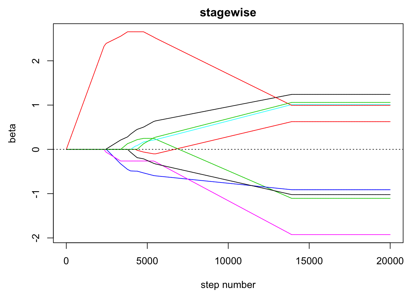

# Sometimes it is useful to visualise the estimated
# coefficients as a function of the sum of the absolute
# values of the coeffs:
matplot(apply(beta, 1, function(x) sum(abs(x))), beta, type = "l", 
    lty = 1, xlab = "sum abs(beta)", ylab = "beta", main = "stagewise")
abline(h = 0, lty = 3)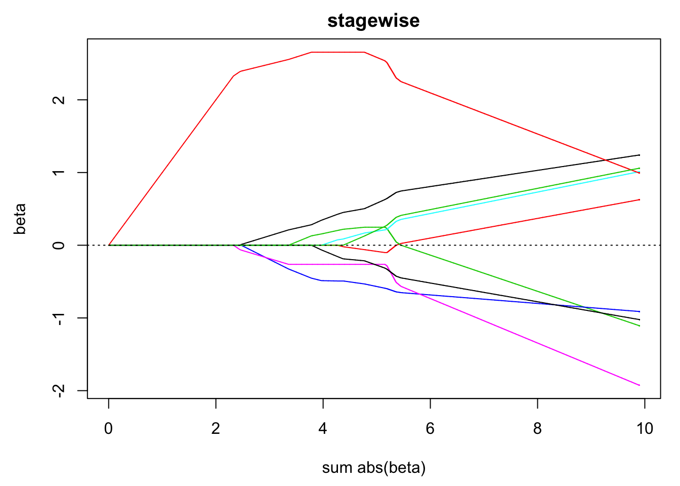

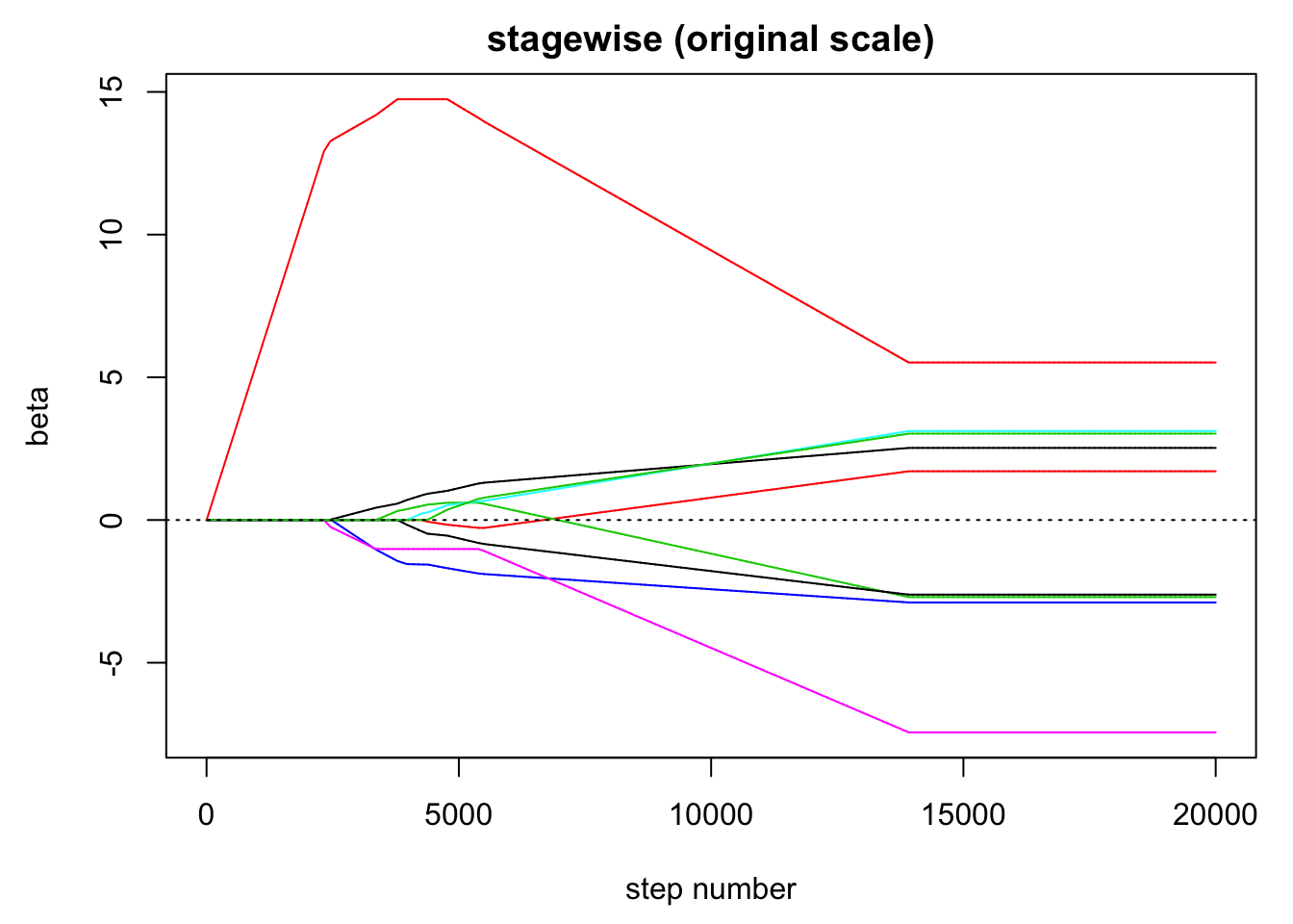
# on the original scale
unscale = scale(beta, center = FALSE, scale = 1/s)
matplot(unscale, type = "l", lty = 1, xlab = "step number", ylab = "beta", 
    main = "stagewise (original scale)")
abline(h = 0, lty = 3)

Lab 2: Exhaustive searching and GLMs

Samuel Müller and Garth Tarr

Learning outcomes

Required R packages:

Crime data

Exercises

Birthweight data

Exercises

Rock-wallabies: cross validation

Advanced: Stagewise selection

Exercise