
Lab 1: Introduction to model selection
Samuel Müller and Garth Tarr
Learning outcomes
- Statistical models
- Assumptions
- Possible models, model space
- What makes a good model
- “Classical” model selection methods
- Residual Sum of Squares
- \(R^2\) and adjusted \(R^2\)
- Information criterion (e.g. AIC, BIC)
- Stepwise search schemes
- Sequential testing
- Backward stepwise methods
Required R packages:
install.packages(c("mplot", "pairsD3", "Hmisc", "d3heatmap",
    "mfp", "dplyr"))
Diabetes example
Efron et al. (2004) introduced the diabetes data set with 442 observations and 11 variables. It is often used as an examplar data set to illustrate new model selection techniques. The following commands will help you get a feel for the data.
data("diabetes", package = "mplot")
# help('diabetes', package='mplot')
str(diabetes)  # structure of the diabetes
## 'data.frame': 442 obs. of 11 variables:
## $ age: int 59 48 72 24 50 23 36 66 60 29 ...
## $ sex: int 2 1 2 1 1 1 2 2 2 1 ...
## $ bmi: num 32.1 21.6 30.5 25.3 23 22.6 22 26.2 32.1 30 ...
## $ map: num 101 87 93 84 101 89 90 114 83 85 ...
## $ tc : int 157 183 156 198 192 139 160 255 179 180 ...
## $ ldl: num 93.2 103.2 93.6 131.4 125.4 ...
## $ hdl: num 38 70 41 40 52 61 50 56 42 43 ...
## $ tch: num 4 3 4 5 4 2 3 4.55 4 4 ...
## $ ltg: num 4.86 3.89 4.67 4.89 4.29 ...
## $ glu: int 87 69 85 89 80 68 82 92 94 88 ...
## $ y : int 151 75 141 206 135 97 138 63 110 310 ...pairs(diabetes) # traditional pairs plot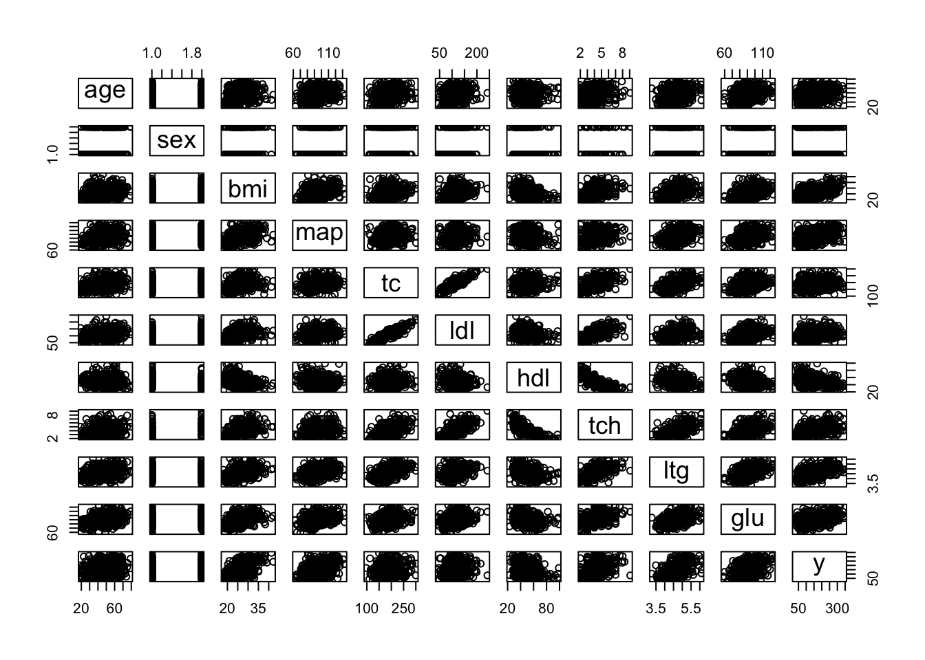
boxplot(diabetes) # always a good idea to check for gross outliers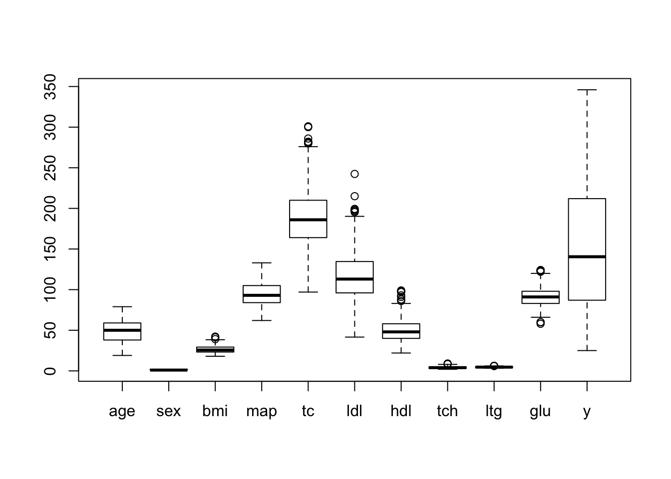
pairsD3::shinypairs(diabetes)  # interactive pairs plot of the data set
d3heatmap::d3heatmap(cor(diabetes))
Hmisc::describe(diabetes, digits = 1)  # summary of the diabetes data
Stepwise model selection
Try to find a couple of good models using the techinques discussed in lectures.
Backwards
M0 = lm(y ~ 1, data = diabetes)  # Null model
M1 = lm(y ~ ., data = diabetes)  # Full model
summary(M1)
##
## Call:
## lm(formula = y ~ ., data = diabetes)
##
## Residuals:
## Min 1Q Median 3Q Max
## -155.827 -38.536 -0.228 37.806 151.353
##
## Coefficients:
## Estimate Std. Error t value Pr(>|t|)
## (Intercept) -334.56714 67.45462 -4.960 1.02e-06 ***
## age -0.03636 0.21704 -0.168 0.867031
## sex -22.85965 5.83582 -3.917 0.000104 ***
## bmi 5.60296 0.71711 7.813 4.30e-14 ***
## map 1.11681 0.22524 4.958 1.02e-06 ***
## tc -1.09000 0.57333 -1.901 0.057948 .
## ldl 0.74645 0.53083 1.406 0.160390
## hdl 0.37200 0.78246 0.475 0.634723
## tch 6.53383 5.95864 1.097 0.273459
## ltg 68.48312 15.66972 4.370 1.56e-05 ***
## glu 0.28012 0.27331 1.025 0.305990
## ---
## Signif. codes:
## 0 '***' 0.001 '**' 0.01 '*' 0.05 '.' 0.1 ' ' 1
##
## Residual standard error: 54.15 on 431 degrees of freedom
## Multiple R-squared: 0.5177, Adjusted R-squared: 0.5066
## F-statistic: 46.27 on 10 and 431 DF, p-value: < 2.2e-16dim(diabetes)## [1] 442 11Try doing backward selecton using AIC first, then using BIC. Do you get the same result?
step.back.bic = step(M1, direction = "backward", trace = FALSE,
    k = log(442))
summary(step.back.bic)
##
## Call:
## lm(formula = y ~ sex + bmi + map + tc + ldl + ltg, data = diabetes)
##
## Residuals:
## Min 1Q Median 3Q Max
## -158.275 -39.476 -2.065 37.219 148.690
##
## Coefficients:
## Estimate Std. Error t value Pr(>|t|)
## (Intercept) -313.7666 25.3848 -12.360 < 2e-16 ***
## sex -21.5910 5.7056 -3.784 0.000176 ***
## bmi 5.7111 0.7073 8.075 6.69e-15 ***
## map 1.1266 0.2158 5.219 2.79e-07 ***
## tc -1.0429 0.2208 -4.724 3.12e-06 ***
## ldl 0.8433 0.2298 3.670 0.000272 ***
## ltg 73.3065 7.3083 10.031 < 2e-16 ***
## ---
## Signif. codes:
## 0 '***' 0.001 '**' 0.01 '*' 0.05 '.' 0.1 ' ' 1
##
## Residual standard error: 54.06 on 435 degrees of freedom
## Multiple R-squared: 0.5149, Adjusted R-squared: 0.5082
## F-statistic: 76.95 on 6 and 435 DF, p-value: < 2.2e-16step.back.aic = step(M1, direction = "backward", trace = FALSE,
k = 2)
summary(step.back.aic)##
## Call:
## lm(formula = y ~ sex + bmi + map + tc + ldl + ltg, data = diabetes)
##
## Residuals:
## Min 1Q Median 3Q Max
## -158.275 -39.476 -2.065 37.219 148.690
##
## Coefficients:
## Estimate Std. Error t value Pr(>|t|)
## (Intercept) -313.7666 25.3848 -12.360 < 2e-16 ***
## sex -21.5910 5.7056 -3.784 0.000176 ***
## bmi 5.7111 0.7073 8.075 6.69e-15 ***
## map 1.1266 0.2158 5.219 2.79e-07 ***
## tc -1.0429 0.2208 -4.724 3.12e-06 ***
## ldl 0.8433 0.2298 3.670 0.000272 ***
## ltg 73.3065 7.3083 10.031 < 2e-16 ***
## ---
## Signif. codes:
## 0 '***' 0.001 '**' 0.01 '*' 0.05 '.' 0.1 ' ' 1
##
## Residual standard error: 54.06 on 435 degrees of freedom
## Multiple R-squared: 0.5149, Adjusted R-squared: 0.5082
## F-statistic: 76.95 on 6 and 435 DF, p-value: < 2.2e-16Forwards
Explore the forwards selection technique, which works very similarly to backwards selection, just set direction = "forward" in the step() function. We will discuss forward selection in more detail in lecture 2. When using direction = "forward" you need to sepecify a scope parameter: scope = list(lower = M0, upper = M1).
step.fwd.bic = step(M0, scope = list(lower = M0, upper = M1),
    direction = "forward", trace = FALSE, k = log(442))
summary(step.fwd.bic)
##
## Call:
## lm(formula = y ~ bmi + ltg + map + tc + sex + ldl, data = diabetes)
##
## Residuals:
## Min 1Q Median 3Q Max
## -158.275 -39.476 -2.065 37.219 148.690
##
## Coefficients:
## Estimate Std. Error t value Pr(>|t|)
## (Intercept) -313.7666 25.3848 -12.360 < 2e-16 ***
## bmi 5.7111 0.7073 8.075 6.69e-15 ***
## ltg 73.3065 7.3083 10.031 < 2e-16 ***
## map 1.1266 0.2158 5.219 2.79e-07 ***
## tc -1.0429 0.2208 -4.724 3.12e-06 ***
## sex -21.5910 5.7056 -3.784 0.000176 ***
## ldl 0.8433 0.2298 3.670 0.000272 ***
## ---
## Signif. codes:
## 0 '***' 0.001 '**' 0.01 '*' 0.05 '.' 0.1 ' ' 1
##
## Residual standard error: 54.06 on 435 degrees of freedom
## Multiple R-squared: 0.5149, Adjusted R-squared: 0.5082
## F-statistic: 76.95 on 6 and 435 DF, p-value: < 2.2e-16step.fwd.aic = step(M0, scope = list(lower = M0, upper = M1),
direction = "forward", trace = FALSE, k = 2)
summary(step.fwd.aic)##
## Call:
## lm(formula = y ~ bmi + ltg + map + tc + sex + ldl, data = diabetes)
##
## Residuals:
## Min 1Q Median 3Q Max
## -158.275 -39.476 -2.065 37.219 148.690
##
## Coefficients:
## Estimate Std. Error t value Pr(>|t|)
## (Intercept) -313.7666 25.3848 -12.360 < 2e-16 ***
## bmi 5.7111 0.7073 8.075 6.69e-15 ***
## ltg 73.3065 7.3083 10.031 < 2e-16 ***
## map 1.1266 0.2158 5.219 2.79e-07 ***
## tc -1.0429 0.2208 -4.724 3.12e-06 ***
## sex -21.5910 5.7056 -3.784 0.000176 ***
## ldl 0.8433 0.2298 3.670 0.000272 ***
## ---
## Signif. codes:
## 0 '***' 0.001 '**' 0.01 '*' 0.05 '.' 0.1 ' ' 1
##
## Residual standard error: 54.06 on 435 degrees of freedom
## Multiple R-squared: 0.5149, Adjusted R-squared: 0.5082
## F-statistic: 76.95 on 6 and 435 DF, p-value: < 2.2e-16The add1 command
Try using the add1() function. The general form is add1(fitted.model, test = "F", scope = M1)
add1(step.fwd.bic, test = "F", scope = M1)## Single term additions
##
## Model:
## y ~ bmi + ltg + map + tc + sex + ldl
## Df Sum of Sq RSS AIC F value Pr(>F)
## <none> 1271494 3534.3
## age 1 10.9 1271483 3536.3 0.0037 0.9515
## hdl 1 394.8 1271099 3536.1 0.1348 0.7137
## tch 1 3686.2 1267808 3535.0 1.2619 0.2619
## glu 1 3532.6 1267961 3535.0 1.2091 0.2721drop1(step.fwd.bic, test = "F")## Single term deletions
##
## Model:
## y ~ bmi + ltg + map + tc + sex + ldl
## Df Sum of Sq RSS AIC F value Pr(>F)
## <none> 1271494 3534.3
## bmi 1 190592 1462086 3594.0 65.205 6.687e-15 ***
## ltg 1 294092 1565586 3624.2 100.614 < 2.2e-16 ***
## map 1 79625 1351119 3559.1 27.241 2.787e-07 ***
## tc 1 65236 1336730 3554.4 22.318 3.123e-06 ***
## sex 1 41856 1313350 3546.6 14.320 0.0001758 ***
## ldl 1 39377 1310871 3545.7 13.472 0.0002723 ***
## ---
## Signif. codes:
## 0 '***' 0.001 '**' 0.01 '*' 0.05 '.' 0.1 ' ' 1Body fat
Your turn to explore with the body fat data set. Using the techniques outlined in the first lecture identify one (or more) models that help explain the body fat percentage of an individual.
data("bodyfat", package = "mplot")
# help('bodyfat', package = 'mplot')
dim(bodyfat)
## [1] 128 15names(bodyfat)## [1] "Id" "Bodyfat" "Age" "Weight" "Height"
## [6] "Neck" "Chest" "Abdo" "Hip" "Thigh"
## [11] "Knee" "Ankle" "Bic" "Fore" "Wrist"bfat = bodyfat[, -1] # remove the ID columnfull.bf = lm(Bodyfat ~ ., data = bfat)
null.bf = lm(Bodyfat ~ 1, data = bfat)
step1 = step(full.bf, direction = "backward")## Start: AIC=373.2
## Bodyfat ~ Age + Weight + Height + Neck + Chest + Abdo + Hip +
## Thigh + Knee + Ankle + Bic + Fore + Wrist
##
## Df Sum of Sq RSS AIC
## - Ankle 1 0.15 1898.7 371.21
## - Age 1 0.76 1899.3 371.25
## - Knee 1 1.47 1900.1 371.29
## - Bic 1 1.59 1900.2 371.30
## - Wrist 1 2.08 1900.7 371.34
## - Thigh 1 4.24 1902.8 371.48
## - Chest 1 5.07 1903.7 371.54
## - Hip 1 8.03 1906.6 371.74
## - Height 1 10.80 1909.4 371.92
## - Weight 1 20.62 1919.2 372.58
## <none> 1898.6 373.20
## - Fore 1 38.19 1936.8 373.74
## - Neck 1 56.38 1955.0 374.94
## - Abdo 1 1088.97 2987.6 429.22
##
## Step: AIC=371.21
## Bodyfat ~ Age + Weight + Height + Neck + Chest + Abdo + Hip +
## Thigh + Knee + Bic + Fore + Wrist
##
## Df Sum of Sq RSS AIC
## - Age 1 0.84 1899.6 369.26
## - Bic 1 1.90 1900.6 369.33
## - Knee 1 1.92 1900.7 369.33
## - Wrist 1 2.64 1901.4 369.38
## - Thigh 1 4.15 1902.9 369.48
## - Chest 1 5.55 1904.3 369.58
## - Hip 1 7.93 1906.7 369.74
## - Height 1 11.90 1910.6 370.01
## - Weight 1 23.59 1922.3 370.79
## <none> 1898.7 371.21
## - Fore 1 38.15 1936.9 371.75
## - Neck 1 57.25 1956.0 373.01
## - Abdo 1 1125.31 3024.1 428.78
##
## Step: AIC=369.26
## Bodyfat ~ Weight + Height + Neck + Chest + Abdo + Hip + Thigh +
## Knee + Bic + Fore + Wrist
##
## Df Sum of Sq RSS AIC
## - Knee 1 1.33 1900.9 367.35
## - Bic 1 1.92 1901.5 367.39
## - Wrist 1 1.93 1901.5 367.39
## - Thigh 1 3.37 1903.0 367.49
## - Chest 1 6.39 1906.0 367.69
## - Hip 1 8.14 1907.7 367.81
## - Height 1 12.16 1911.7 368.08
## - Weight 1 27.13 1926.7 369.08
## <none> 1899.6 369.26
## - Fore 1 37.85 1937.4 369.79
## - Neck 1 56.57 1956.1 371.02
## - Abdo 1 1346.09 3245.7 435.83
##
## Step: AIC=367.35
## Bodyfat ~ Weight + Height + Neck + Chest + Abdo + Hip + Thigh +
## Bic + Fore + Wrist
##
## Df Sum of Sq RSS AIC
## - Bic 1 2.03 1902.9 365.49
## - Thigh 1 2.63 1903.5 365.53
## - Wrist 1 2.73 1903.6 365.53
## - Chest 1 7.05 1908.0 365.82
## - Hip 1 7.62 1908.5 365.86
## - Height 1 11.23 1912.1 366.11
## <none> 1900.9 367.35
## - Weight 1 30.51 1931.4 367.39
## - Fore 1 39.05 1940.0 367.95
## - Neck 1 55.47 1956.4 369.03
## - Abdo 1 1345.48 3246.4 433.86
##
## Step: AIC=365.49
## Bodyfat ~ Weight + Height + Neck + Chest + Abdo + Hip + Thigh +
## Fore + Wrist
##
## Df Sum of Sq RSS AIC
## - Wrist 1 2.79 1905.7 363.68
## - Thigh 1 4.63 1907.6 363.80
## - Hip 1 7.50 1910.4 363.99
## - Chest 1 7.55 1910.5 363.99
## - Height 1 10.21 1913.1 364.17
## - Weight 1 29.27 1932.2 365.44
## <none> 1902.9 365.49
## - Fore 1 50.40 1953.3 366.83
## - Neck 1 54.04 1957.0 367.07
## - Abdo 1 1353.15 3256.1 432.24
##
## Step: AIC=363.68
## Bodyfat ~ Weight + Height + Neck + Chest + Abdo + Hip + Thigh +
## Fore
##
## Df Sum of Sq RSS AIC
## - Thigh 1 7.00 1912.7 362.14
## - Hip 1 8.01 1913.7 362.21
## - Chest 1 9.29 1915.0 362.30
## - Height 1 13.86 1919.6 362.60
## <none> 1905.7 363.68
## - Weight 1 36.34 1942.1 364.09
## - Fore 1 50.12 1955.8 365.00
## - Neck 1 79.05 1984.8 366.88
## - Abdo 1 1372.77 3278.5 431.12
##
## Step: AIC=362.14
## Bodyfat ~ Weight + Height + Neck + Chest + Abdo + Hip + Fore
##
## Df Sum of Sq RSS AIC
## - Hip 1 4.42 1917.1 360.44
## - Chest 1 5.38 1918.1 360.50
## - Height 1 8.62 1921.3 360.72
## - Weight 1 29.49 1942.2 362.10
## <none> 1912.7 362.14
## - Fore 1 51.53 1964.3 363.55
## - Neck 1 80.80 1993.5 365.44
## - Abdo 1 1372.41 3285.1 429.38
##
## Step: AIC=360.44
## Bodyfat ~ Weight + Height + Neck + Chest + Abdo + Fore
##
## Df Sum of Sq RSS AIC
## - Chest 1 12.90 1930.0 359.30
## - Height 1 17.44 1934.6 359.60
## <none> 1917.1 360.44
## - Fore 1 59.51 1976.6 362.35
## - Neck 1 76.42 1993.6 363.44
## - Weight 1 117.40 2034.5 366.05
## - Abdo 1 1370.48 3287.6 427.47
##
## Step: AIC=359.3
## Bodyfat ~ Weight + Height + Neck + Abdo + Fore
##
## Df Sum of Sq RSS AIC
## - Height 1 9.06 1939.1 357.90
## <none> 1930.0 359.30
## - Fore 1 59.13 1989.2 361.16
## - Neck 1 74.35 2004.4 362.14
## - Weight 1 107.93 2038.0 364.26
## - Abdo 1 1679.52 3609.6 437.43
##
## Step: AIC=357.9
## Bodyfat ~ Weight + Neck + Abdo + Fore
##
## Df Sum of Sq RSS AIC
## <none> 1939.1 357.90
## - Fore 1 52.30 1991.4 359.30
## - Neck 1 85.21 2024.3 361.40
## - Weight 1 133.93 2073.0 364.45
## - Abdo 1 2283.87 4223.0 455.52step2 = step(null.bf, scope = list(lower = null.bf, upper = full.bf),
direction = "forward")## Start: AIC=525.59
## Bodyfat ~ 1
##
## Df Sum of Sq RSS AIC
## + Abdo 1 5376.2 2274.9 372.34
## + Chest 1 4166.5 3484.7 426.93
## + Weight 1 3348.3 4302.9 453.92
## + Hip 1 3011.2 4640.0 463.58
## + Thigh 1 2089.3 5561.8 486.77
## + Bic 1 1848.4 5802.8 492.20
## + Knee 1 1819.1 5832.0 492.84
## + Neck 1 1652.8 5998.3 496.44
## + Wrist 1 1350.2 6300.9 502.74
## + Ankle 1 989.0 6662.2 509.88
## + Fore 1 886.5 6764.7 511.83
## + Age 1 495.1 7156.1 519.03
## + Height 1 175.3 7475.8 524.63
## <none> 7651.2 525.59
##
## Step: AIC=372.34
## Bodyfat ~ Abdo
##
## Df Sum of Sq RSS AIC
## + Weight 1 228.962 2046.0 360.76
## + Neck 1 191.968 2082.9 363.06
## + Hip 1 180.253 2094.7 363.78
## + Wrist 1 134.105 2140.8 366.56
## + Ankle 1 119.710 2155.2 367.42
## + Knee 1 113.440 2161.5 367.79
## + Thigh 1 94.488 2180.4 368.91
## + Height 1 64.441 2210.5 370.66
## + Bic 1 53.419 2221.5 371.30
## <none> 2274.9 372.34
## + Chest 1 27.282 2247.6 372.80
## + Age 1 20.550 2254.4 373.18
## + Fore 1 15.172 2259.8 373.49
##
## Step: AIC=360.76
## Bodyfat ~ Abdo + Weight
##
## Df Sum of Sq RSS AIC
## + Neck 1 54.563 1991.4 359.30
## + Wrist 1 33.470 2012.5 360.65
## <none> 2046.0 360.76
## + Fore 1 21.648 2024.3 361.40
## + Hip 1 10.725 2035.2 362.09
## + Height 1 9.781 2036.2 362.15
## + Ankle 1 3.584 2042.4 362.54
## + Chest 1 2.967 2043.0 362.58
## + Age 1 2.596 2043.4 362.60
## + Bic 1 2.257 2043.7 362.62
## + Knee 1 1.891 2044.1 362.65
## + Thigh 1 0.161 2045.8 362.75
##
## Step: AIC=359.3
## Bodyfat ~ Abdo + Weight + Neck
##
## Df Sum of Sq RSS AIC
## + Fore 1 52.296 1939.1 357.90
## <none> 1991.4 359.30
## + Hip 1 24.094 1967.3 359.75
## + Bic 1 9.256 1982.1 360.71
## + Chest 1 7.046 1984.3 360.85
## + Wrist 1 6.772 1984.6 360.87
## + Ankle 1 5.096 1986.3 360.98
## + Knee 1 3.707 1987.7 361.07
## + Height 1 2.231 1989.2 361.16
## + Thigh 1 0.423 1991.0 361.28
## + Age 1 0.010 1991.4 361.30
##
## Step: AIC=357.9
## Bodyfat ~ Abdo + Weight + Neck + Fore
##
## Df Sum of Sq RSS AIC
## <none> 1939.1 357.90
## + Hip 1 16.7889 1922.3 358.78
## + Height 1 9.0643 1930.0 359.30
## + Wrist 1 8.3637 1930.7 359.34
## + Ankle 1 7.4509 1931.7 359.40
## + Chest 1 4.5251 1934.6 359.60
## + Knee 1 1.4926 1937.6 359.80
## + Thigh 1 1.0270 1938.1 359.83
## + Bic 1 0.3077 1938.8 359.88
## + Age 1 0.2046 1938.9 359.88summary(step1)##
## Call:
## lm(formula = Bodyfat ~ Weight + Neck + Abdo + Fore, data = bfat)
##
## Residuals:
## Min 1Q Median 3Q Max
## -9.1637 -2.8476 0.0877 2.7522 8.3342
##
## Coefficients:
## Estimate Std. Error t value Pr(>|t|)
## (Intercept) -41.88325 8.30967 -5.040 1.62e-06 ***
## Weight -0.22932 0.07868 -2.915 0.00423 **
## Neck -0.61856 0.26606 -2.325 0.02172 *
## Abdo 0.98046 0.08146 12.036 < 2e-16 ***
## Fore 0.43409 0.23834 1.821 0.07099 .
## ---
## Signif. codes:
## 0 '***' 0.001 '**' 0.01 '*' 0.05 '.' 0.1 ' ' 1
##
## Residual standard error: 3.971 on 123 degrees of freedom
## Multiple R-squared: 0.7466, Adjusted R-squared: 0.7383
## F-statistic: 90.58 on 4 and 123 DF, p-value: < 2.2e-16summary(step2)##
## Call:
## lm(formula = Bodyfat ~ Abdo + Weight + Neck + Fore, data = bfat)
##
## Residuals:
## Min 1Q Median 3Q Max
## -9.1637 -2.8476 0.0877 2.7522 8.3342
##
## Coefficients:
## Estimate Std. Error t value Pr(>|t|)
## (Intercept) -41.88325 8.30967 -5.040 1.62e-06 ***
## Abdo 0.98046 0.08146 12.036 < 2e-16 ***
## Weight -0.22932 0.07868 -2.915 0.00423 **
## Neck -0.61856 0.26606 -2.325 0.02172 *
## Fore 0.43409 0.23834 1.821 0.07099 .
## ---
## Signif. codes:
## 0 '***' 0.001 '**' 0.01 '*' 0.05 '.' 0.1 ' ' 1
##
## Residual standard error: 3.971 on 123 degrees of freedom
## Multiple R-squared: 0.7466, Adjusted R-squared: 0.7383
## F-statistic: 90.58 on 4 and 123 DF, p-value: < 2.2e-16Both forward and backward stepwise select a model with Fore, Neck, Weight and Abdo. It does look to be substantially better than a simple linear regression of Bodyfat on Abdo (the best simple linear regression model).
slr.bf = lm(Bodyfat ~ Abdo, data = bfat)
summary(slr.bf)
##
## Call:
## lm(formula = Bodyfat ~ Abdo, data = bfat)
##
## Residuals:
## Min 1Q Median 3Q Max
## -10.3542 -2.9928 0.2191 2.4967 10.0106
##
## Coefficients:
## Estimate Std. Error t value Pr(>|t|)
## (Intercept) -43.19058 3.63431 -11.88 <2e-16 ***
## Abdo 0.67411 0.03907 17.26 <2e-16 ***
## ---
## Signif. codes:
## 0 '***' 0.001 '**' 0.01 '*' 0.05 '.' 0.1 ' ' 1
##
## Residual standard error: 4.249 on 126 degrees of freedom
## Multiple R-squared: 0.7027, Adjusted R-squared: 0.7003
## F-statistic: 297.8 on 1 and 126 DF, p-value: < 2.2e-16summary(slr.bf)$adj.r.squared## [1] 0.7003103summary(step1)$adj.r.squared## [1] 0.7383196AIC(slr.bf)## [1] 737.59AIC(step1)## [1] 723.1457anova(slr.bf, step1)## Analysis of Variance Table
##
## Model 1: Bodyfat ~ Abdo
## Model 2: Bodyfat ~ Weight + Neck + Abdo + Fore
## Res.Df RSS Df Sum of Sq F Pr(>F)
## 1 126 2274.9
## 2 123 1939.1 3 335.82 7.1005 0.0001936 ***
## ---
## Signif. codes:
## 0 '***' 0.001 '**' 0.01 '*' 0.05 '.' 0.1 ' ' 1Advanced: Leave-one-out cross-validation
The leave-one-out cross-validation statistic (or prediction residual sum of squares - PRESS) is, \[CV = \frac{1}{n}\sum_{i=1}^{n}e_{[i]}^2,\] where \(e_{[i]} = y_i - \hat{y}_{[i]}\) for \(i=1,\ldots,n\) and \(\hat{y}_{[i]}\) is the predicted value obtained when the model is estimated after deleting the \(i\)th observation.
Program your own leave-one-out CV function and use it to evaluate between competing models from the body fat or diabetes examples. Hint: you might want to use the update() function: refit = update(fit, subset = index != i) where index and i are as defined in the outline of a function below.
loocv = function(fit){
  n = length(fit$residuals)
  yvar = fit$model[,1]
  index = 1:n
  e = rep(NA, n)
  for (i in index) {
    refit =
    pred =
    e[i] =
  }
  return(mean(e^2))
}
loocv = function(fit) {
n = length(fit$residuals)
yvar = fit$model[, 1]
index = 1:n
e = rep(NA, n)
for (i in index) {
refit = update(fit, subset = index != i)
pred = predict(refit, dplyr::slice(fit$model, i))
e[i] = yvar[i] - pred
}
return(mean(e^2))
}Diabetes
Compare between the selected stepwise model and a simpler model simple.model = lm(y~bmi+ltg+map, data = diabetes). We’ll see justification for this simpler model in lab 4.
simple.model = lm(y ~ bmi + ltg + map, data = diabetes)
step.model = lm(y ~ bmi + ltg + map + tc + sex + ldl, data = diabetes)
loocv(step.model)
## [1] 2967.821loocv(simple.model)## [1] 3139.562summary(step.model)$adj.r.square## [1] 0.5081925summary(simple.model)$adj.r.square## [1] 0.4765214Body fat
Compare between the chosen stepwise model and the simple linear regression of Bodyfat on Abdo.
loocv(slr.bf)## [1] 18.38165step.bf = lm(step1)
loocv(step.bf)## [1] 16.33509Optional extra: Confirm (numerically) that \[CV = \frac{1}{n}\sum_{i=1}^{n}\left(\frac{e_i}{1-h_i}\right)^2,\] where \(e_i\) are the residuals from the model estimated with the full data set and \(h_i\) are the diagonal elements of the hat matrix for the full data set, \(\mathbf{H} = \mathbf{X}(\mathbf{X}^\top\mathbf{X})^{-1}\mathbf{X}^\top\). The implication here is that you do not need to estimate all \(n\) submodels. Hint: lm.influence(fit)$h extracts the diagonal of the hat matrix and residuals(fit) extracts the residuals for the lm object fit.
loocv.h = function(fit) {
  h =
  e =
  return(            )
}
loocv.h = function(fit) {
h = lm.influence(fit)$h
e = residuals(fit)
return(mean((e/(1 - h))^2))
}loocv.h(slr.bf)## [1] 18.38165loocv(slr.bf)## [1] 18.38165loocv.h(step.bf)## [1] 16.33509loocv(step.bf)## [1] 16.33509Prediction error
The body fat data included in the mplot package is a subset of a larger data set, which can be found in the mfp package. You could consider the subset in the mplot package to be a training set.
data("bodyfat", package = "mplot")
head(bodyfat)
## Id Bodyfat Age Weight Height Neck Chest Abdo Hip Thigh
## 1 69 6.3 54 70.42 69.25 37.5 89.3 78.4 96.1 56.0
## 2 98 11.3 50 73.71 66.50 38.7 99.4 86.7 96.2 62.1
## 3 146 14.2 24 70.76 70.75 35.7 92.7 81.9 95.3 56.4
## 4 227 14.8 55 76.88 68.25 37.2 101.7 91.1 97.1 56.6
## 5 53 8.0 51 62.26 67.75 36.5 89.7 82.0 89.1 49.3
## 6 223 11.5 54 73.37 67.50 37.4 94.2 87.6 95.6 59.7
## Knee Ankle Bic Fore Wrist
## 1 37.4 22.4 32.6 28.1 18.1
## 2 39.3 23.3 30.6 27.8 18.2
## 3 36.5 22.0 33.5 28.3 17.3
## 4 38.5 22.6 33.4 29.3 18.8
## 5 33.7 21.4 29.6 26.0 16.9
## 6 40.2 23.4 27.9 27.0 17.8nms = names(bodyfat)
training.id = bodyfat$Id
# install.pacakges('mfp')
data("bodyfat", package = "mfp")
names(bodyfat)## [1] "case" "brozek" "siri" "density" "age"
## [6] "weight" "height" "neck" "chest" "abdomen"
## [11] "hip" "thigh" "knee" "ankle" "biceps"
## [16] "forearm" "wrist"# there were two additional measures of body fat, remove
# these:
bfat.full = subset(bodyfat, select = -c(brozek, density))
bfat.full[training.id[1:6], ]## case siri age weight height neck chest abdomen hip
## 69 69 6.3 54 155.25 69.25 37.5 89.3 78.4 96.1
## 98 98 11.3 50 162.50 66.50 38.7 99.4 86.7 96.2
## 146 146 14.2 24 156.00 70.75 35.7 92.7 81.9 95.3
## 227 227 14.8 55 169.50 68.25 37.2 101.7 91.1 97.1
## 53 53 8.0 51 137.25 67.75 36.5 89.7 82.0 89.1
## 223 223 11.5 54 161.75 67.50 37.4 94.2 87.6 95.6
## thigh knee ankle biceps forearm wrist
## 69 56.0 37.4 22.4 32.6 28.1 18.1
## 98 62.1 39.3 23.3 30.6 27.8 18.2
## 146 56.4 36.5 22.0 33.5 28.3 17.3
## 227 56.6 38.5 22.6 33.4 29.3 18.8
## 53 49.3 33.7 21.4 29.6 26.0 16.9
## 223 59.7 40.2 23.4 27.9 27.0 17.8# ensure common naming conventions:
colnames(bfat.full) = nms
training = is.element(bfat.full$Id, training.id)
bfat.train = bfat.full[training, -1]
bfat.validate = bfat.full[!training, -1]
dim(bfat.train)## [1] 128 14dim(bfat.validate)## [1] 124 14boxplot(bfat.validate, horizontal = TRUE, las = 1)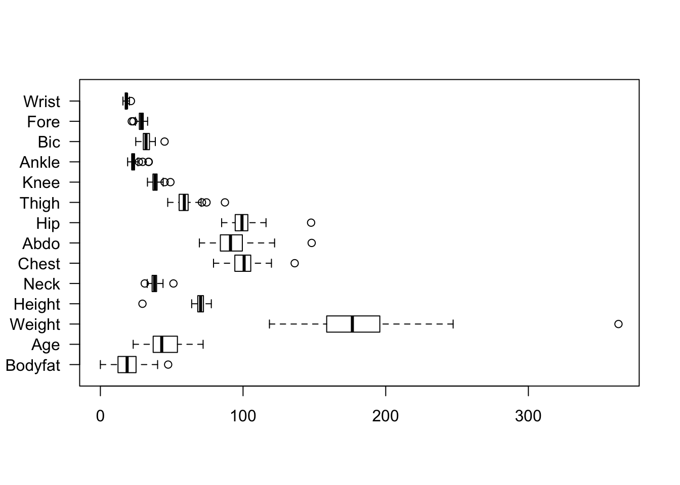
# need to reestimate the models on the training data set only
# because weight is in lbs no kg
slr.bf = lm(Bodyfat ~ Abdo, data = bfat.train)
step.bf = lm(Bodyfat ~ Abdo + Fore + Neck + Weight, data = bfat.train)
Evaluate the performance of the various models identified earlier against the validation data (hint: use the predict() function).
pred.slr = predict(slr.bf, newdata = bfat.validate)
pred.step = predict(step.bf, newdata = bfat.validate)
slr.err = pred.slr - bfat.validate$Bodyfat
step.err = pred.step - bfat.validate$Bodyfat
boxplot(slr.err, step.err, ylab = "Prediction error", names = c("SLR",
    "Step"))
par(mfrow = c(1, 2), mar = c(4.1, 4.1, 0.1, 0.1))
ylims = c(-25, 25)
plot(slr.err, ylab = "SLR prediction error", ylim = ylims)
plot(step.err, ylab = "Step prediction error", ylim = ylims)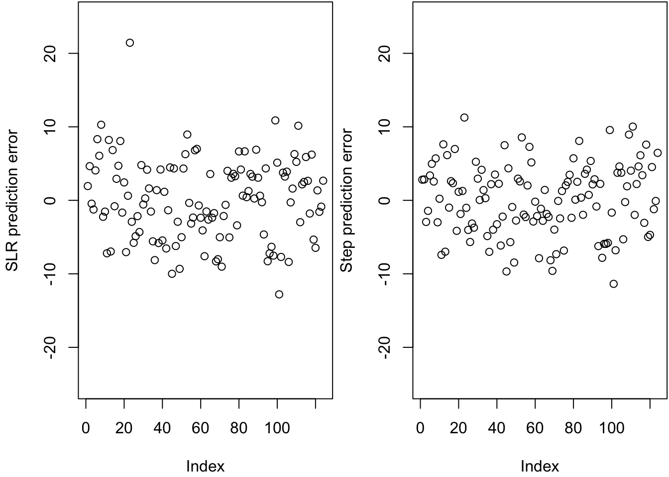
# sum of squared prediction errors:
c(sum(slr.err^2), sum(step.err^2))
## [1] 3726.703 2879.092# mean square prediction error:
c(mean(slr.err^2), mean(step.err^2))## [1] 30.05405 23.21849Note that there are some unusual observations in the validation data set bfat.validate. You might consider identifying and removing those for the purposes of model selection.
which.max(bfat.validate$Weight)## [1] 23which.min(bfat.validate$Height)## [1] 25bfat.validate2 = bfat.validate[-c(23, 25), ]
boxplot(bfat.validate2, horizontal = TRUE, las = 1)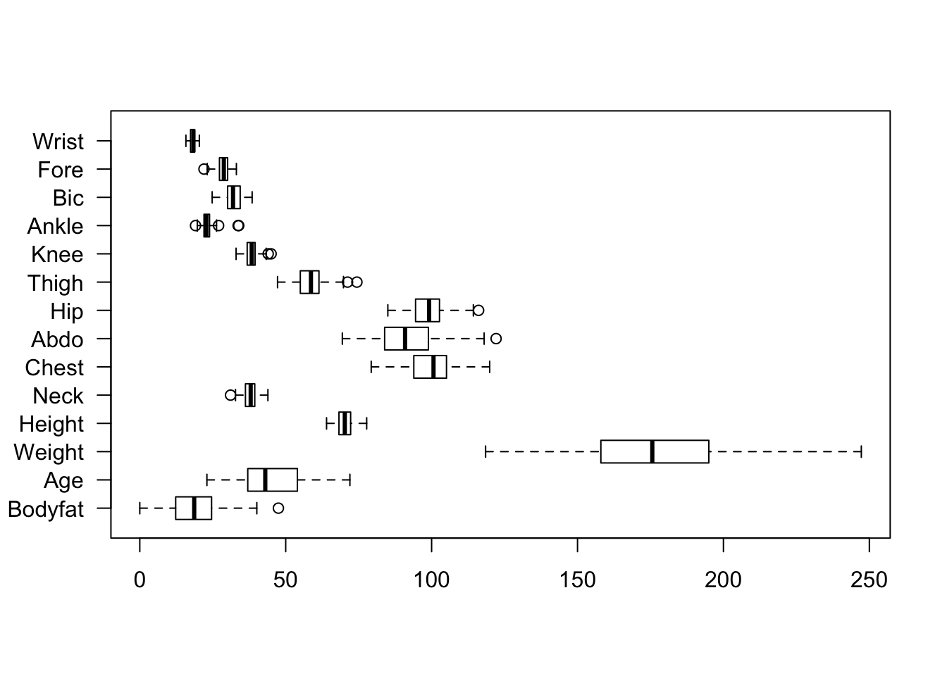
pred.slr = predict(slr.bf, newdata = bfat.validate2)
pred.step = predict(step.bf, newdata = bfat.validate2)
slr.err = pred.slr - bfat.validate2$Bodyfat
step.err = pred.step - bfat.validate2$Bodyfat
boxplot(slr.err, step.err, ylab = "Prediction error", names = c("SLR",
    "Step"))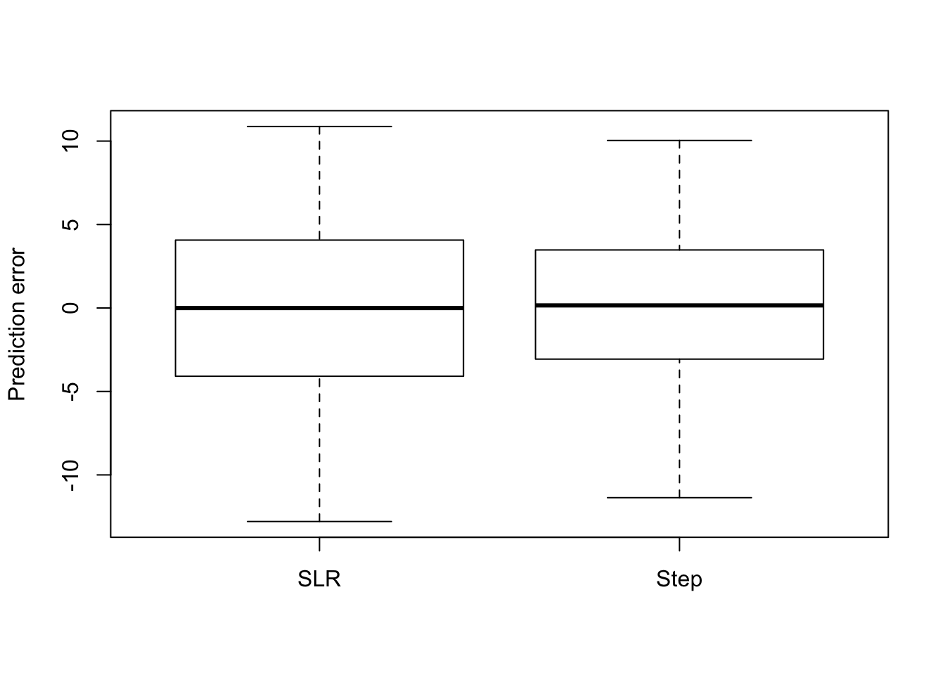
par(mfrow = c(1, 2), mar = c(4.1, 4.1, 0.1, 0.1))
ylims = c(-12, 12)
plot(slr.err, ylab = "SLR prediction error", ylim = ylims)
plot(step.err, ylab = "Step prediction error", ylim = ylims)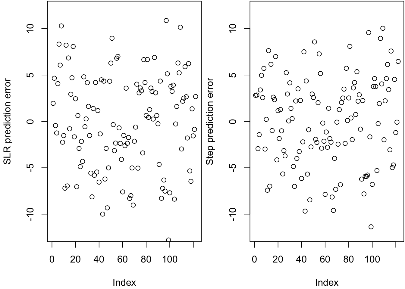
# sum of squared prediction errors:
c(sum(slr.err^2), sum(step.err^2))
## [1] 3233.376 2735.965# mean square prediction error:
c(mean(slr.err^2), mean(step.err^2))## [1] 26.50309 22.42595The stepwise model still performs better than the simple linear regression, though the mean square prediction error of the simple linear regression is substantially reduced when the unusual observations are removed from the validation training set.
References
- Efron B, Hastie T, Johnstone I and Tibshirani R (2004). Least angle regression. The Annals of Statistics 32(2): 407-499. doi:10.1214/009053604000000067
- Johnson RW (1996). Fitting Percentage of Body Fat to Simple Body Measurements. Journal of Statistics Education (4)1, http://www.amstat.org/publications/jse/v4n1/datasets.johnson.html
- Tarr G (2015). pairsD3: D3 scatterplot matrices. R package version 0.1.1, http://github.com/garthtarr/pairsD3