The Lasso Distribution

Provides functions related to the Lasso distribution, including the normalizing constant, probability density function, cumulative distribution function, quantile function, and random number generation for given parameters a, b, and c. Additional utilities include the Mills ratio, expected value, and variance of the distribution. The package also implements modified versions of the Hans and Park–Casella Gibbs sampling algorithms for Bayesian Lasso regression.

Usage

zlasso(a, b, c, logarithm)
dlasso(x, a, b, c, logarithm)
plasso(q, a, b, c)
qlasso(p, a, b, c)
rlasso(n, a, b, c)
elasso(a, b, c)
vlasso(a, b, c)
mlasso(a, b, c)
MillsRatio(d)
Modified_Hans_Gibbs(X, y, a1, b1, u1, v1,
              nsamples, beta_init, lambda_init, sigma2_init, verbose)
Modified_PC_Gibbs(X, y, a1, b1, u1, v1, 
              nsamples, lambda_init, sigma2_init, verbose)

Arguments

x, q: Vector of quantiles (vectorized).
p: Vector of probabilities.
a: Vector of precision parameter which must be non-negative.
b: Vector of off set parameter.
c: Vector of tuning parameter which must be non-negative values.
n: Number of observations.
logarithm: Logical. If TRUE, probabilities are returned on the log scale.
d: A scalar numeric value. Represents the point at which the Mills ratio is evaluated.
X: Design matrix (numeric matrix).
y: Response vector (numeric vector).
a1: Shape parameter of the prior on $\lambda^2$.
b1: Rate parameter of the prior on $\lambda^2$.
u1: Shape parameter of the prior on $\sigma^2$.
v1: Rate parameter of the prior on $\sigma^2$.
nsamples: Number of Gibbs samples to draw.
beta_init: Initial value for the model parameter $\beta$.
lambda_init: Initial value for the shrinkage parameter $\lambda^2$.
sigma2_init: Initial value for the error variance $\sigma^2$.
verbose: Integer. If greater than 0, progress is printed every verbose iterations during sampling. Set to 0 to suppress output.

Value

zlasso, dlasso, plasso, qlasso, rlasso, elasso, vlasso, mlasso, MillsRatio: return the corresponding scalar or vector values related to the Lasso distribution and a numeric value representing the Mills ratio.
Modified_Hans_Gibbs: returns a list containing:
mBeta

Matrix of MCMC samples for the regression coefficients $\beta$, with nsamples rows and p columns.

vsigma2

Vector of MCMC samples for the error variance $\sigma^2$.

vlambda2

Vector of MCMC samples for the shrinkage parameter $\lambda^2$.

mA

Matrix of sampled values for parameter $a_j$ of the Lasso distribution for each $\beta_j$.

mB

Matrix of sampled values for parameter $b_j$ of the Lasso distribution for each $\beta_j$.

mC

Matrix of sampled values for parameter $c_j$ of the Lasso distribution for each $\beta_j$.
Modified_PC_Gibbs: returns a list containing:
mBeta

Matrix of MCMC samples for the regression coefficients $\beta$.

vsigma2

Vector of MCMC samples for the error variance $\sigma^2$.

vlambda2

Vector of MCMC samples for the shrinkage parameter $\lambda^2$.

mM

Matrix of estimated means of the full conditional distributions of each $\beta_j$.

mV

Matrix of estimated variances of the full conditional distributions of each $\beta_j$.

va_til

Vector of estimated shape parameters for the full conditional inverse-gamma distribution of $\sigma^2$.

vb_til

Vector of estimated rate parameters for the full conditional inverse-gamma distribution of $\sigma^2$.

vu_til

Vector of estimated shape parameters for the full conditional inverse-gamma distribution of $\lambda^2$.

vv_til

Vector of estimated rate parameters for the full conditional inverse-gamma distribution of $\lambda^2$.

Details

If $X \sim \text{Lasso}(a, b, c)$ then its density function is: $$ p(x;a,b,c) = Z^{-1} \exp\left(-\frac{1}{2} a x^2 + bx - c|x| \right) $$ where $x \in \mathbb{R}$, $a > 0$, $b \in \mathbb{R}$, $c > 0$, and $Z$ is the normalizing constant.

More details are included for the CDF, quantile function, and normalizing constant in the original documentation.

Examples

a <- 2; b <- 1; c <- 3
x <- seq(-3, 3, length.out = 1000)
plot(x, dlasso(x, a, b, c, logarithm = FALSE), type = 'l')


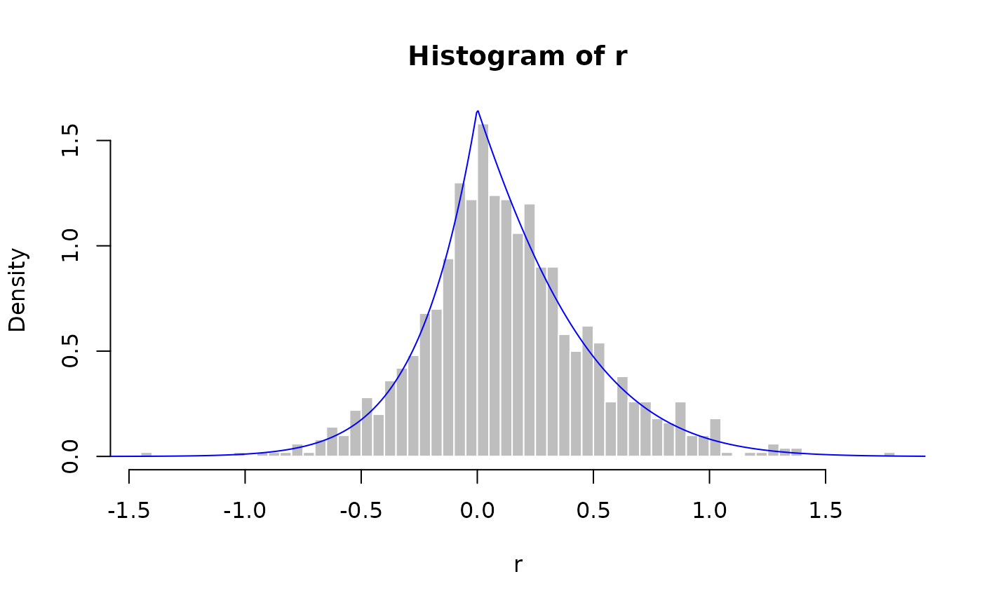
r <- rlasso(1000, a, b, c)
hist(r, breaks = 50, probability = TRUE, col = "grey", border = "white")
lines(x, dlasso(x, a, b, c, logarithm = FALSE), col = "blue")


plasso(0, a, b, c)
#> [1] 0.3739435
qlasso(0.25, a, b, c)
#> [1] -0.08945799
elasso(a, b, c)
#> [1] 0.1218306
vlasso(a, b, c)
#> [1] 0.1287739
mlasso(a, b, c)
#> [1] 0
MillsRatio(2)
#> [1] 0.4213692




# The Modified_Hans_Gibbs() function uses the Lasso distribution to draw 
# samples from the full conditional distribution of the regression coefficients.

y <- 1:20
X <- matrix(c(1:20,12:31,7:26),20,3,byrow = TRUE)

a1 <- b1 <- u1 <- v1 <- 0.01
sigma2_init <- 1
lambda_init <- 0.1
beta_init <- rep(1, ncol(X))
nsamples <- 1000
verbose <- 100

Output_Hans <- Modified_Hans_Gibbs(
                X, y, a1, b1, u1, v1,
                nsamples, beta_init, lambda_init, sigma2_init, verbose
)
#> iter: 0 lambda2: 111.808 sigma2: 87.5523
#> iter: 100 lambda2: 78.3137 sigma2: 31.5026
#> iter: 200 lambda2: 82.2531 sigma2: 22.8744
#> iter: 300 lambda2: 43.4028 sigma2: 16.3699
#> iter: 400 lambda2: 93.2793 sigma2: 21.5296
#> iter: 500 lambda2: 16.2335 sigma2: 25.1914
#> iter: 600 lambda2: 74.3442 sigma2: 10.7202
#> iter: 700 lambda2: 43.4173 sigma2: 20.7042
#> iter: 800 lambda2: 13.0825 sigma2: 26.2766
#> iter: 900 lambda2: 8.89624 sigma2: 15.0216

colMeans(Output_Hans$mBeta)
#> [1] 0.300507310 0.003085177 0.321644003
mean(Output_Hans$vlambda2)
#> [1] 71.41197


Output_PC <- Modified_PC_Gibbs(
               X, y, a1, b1, u1, v1, 
               nsamples, lambda_init, sigma2_init, verbose)
#> iter: 0
#> iter: 100
#> iter: 200
#> iter: 300
#> iter: 400
#> iter: 500
#> iter: 600
#> iter: 700
#> iter: 800
#> iter: 900

colMeans(Output_PC$mBeta)
#> [1]  0.31996577 -0.09120189  0.38965795
mean(Output_PC$vlambda2)
#> [1] 69.64793

Usage

Arguments

Value

Details

See also

Examples